Econ 616: Problem Set 1
Problem 1
Let \(\phi (z) \equiv 1 - \phi_1 z - \phi_2 z^2\). What we need to show is the solution of the equation \(\phi ( z) =0\) lies outside of unit circle. Let \(z_1\) and \(z_2\) be the solutions of \(\phi (z) =0\).
Case 1: Suppose \(\phi _{1}^{2}+4\phi _{2}\leq 0\). Then we have either \(z_{1}=z_{2}\) or that \(z_{1}\) and \(z_{2}\) are complex numbers and conjugate of each other. In any case the norm of the solution is given by \(\sqrt{\left\vert \frac{1}{\phi _{2}}\right\vert }\). Hence the condition is \(|\phi_{2}|<1\).
Case 2: Suppose \(\phi_1^2 + 4 \phi_2 > 0\). Now both solutions are real number. Suppose \(\phi_2 =0\). This is AR(1) model and the condition is \(|\phi_1 | <1\). Suppose \(\phi_2 \neq 0\). It would be easier to analyze the equation \(\psi(z) =0\) where \(\psi(z) \equiv z^2 + \frac{\phi_1}{\phi_2}z - \frac{1}{\phi_2}\) which has the same solutions as \(\phi(z) =0\). If \(\phi_2 <0\), then the conditions are \(\psi(1 )> 0\) and \(\psi(-1) >0\) which means that \(\phi_2+\phi_1 <1\) and \(\phi_2 - \phi_1 <1\). If $φ_2 > 0 $, then the conditions are \(\psi(1 ) < 0\) and \(\psi(-1) <0\) which means that \(\phi_2+\phi_1 <1\) and \(\phi_2 - \phi_1 <1\).
Combining all, we have
\begin{eqnarray*} \phi _{1}+\phi _{2}<1,\quad \phi _{2}-\phi _{1}<1\mbox{ and }\phi _{2}>-1. \end{eqnarray*}
Problem 2
Multiplying both sides of the equation by \(y_{t-j}\), we have
\begin{eqnarray*} y_{t}y_{t-j}=\sum_{i=1}^{p}\phi _{i}y_{t-i}y_{t-j}+\epsilon _{t}y_{t-j}. \end{eqnarray*}% Taking the expectation, we have \begin{eqnarray*} E(y_{t}y_{t-j})=\sum_{i=1}^{p}\phi _{i}E(y_{t-i}y_{t-j})+E(\epsilon _{t}y_{t-j}). \end{eqnarray*}% Or we can rewrite the above as \begin{eqnarray*} \gamma _{yy,j}=\sum_{i=1}^{p}\phi _{i}\gamma _{yy,|i-j|}+E(\epsilon _{t}y_{t-j}). \end{eqnarray*}
For \(j=0\), \(E(\epsilon _{t}y_{t-j})=E(\epsilon _{t}y_{t})=E(\epsilon _{t}^{2})=\sigma _{\epsilon }^{2}\) which gives the first equation. For \(% j=1,\dots ,p\), \(E(\epsilon _{t}y_{t-j})=0\) which gives the rest.
For the AR(3) process in Problem 2, we have
\begin{eqnarray*} 1 &=& \gamma_{yy,0}-(1.3\gamma_{yy,1}-0.9\gamma_{yy,2}+0.3\gamma_{yy,3}) \\ 0 &=& 1.3\gamma_{yy,0}-\gamma_{yy,1}+(-0.9\gamma_{yy,1}+0.3\gamma_{yy,2}) \\ 0 &=& -0.9\gamma_{yy,0}-\gamma_{yy,2}+(1.3\gamma_{yy,1}+0.3\gamma_{yy,1})\\ 0 &=& 0.3\gamma_{yy,0}-\gamma_{yy,3}+(1.3\gamma_{yy,2}-0.9\gamma_{yy,1}) \end{eqnarray*}
Solutions to this system of equations are
\(\gamma_{yy,0}=3.38\quad \gamma_{yy,1}=2.45\qquad \gamma_{yy,2}=0.88\qquad \gamma_{yy,3}=-0.48\)
Problem 3
See jupyter notebook
Problem 4
The least squares estimates can be written as:
\begin{align} \hat\rho_{LS} = \rho + \left(\sum_{t=2}^T y_{t-1}^2\right)^{-1}\sum_{t=2}^T \epsilon_t y_{t-1} \end{align}
Consider an alternative representation of \(y_t\).
\begin{align} t \mbox{ even} &:& y_t &= y_t^e = \rho^2 y_t^e + \sigma\epsilon_t + \rho\alpha\sigma\epsilon_{t-1} \nonumber \\ t \mbox{ odd} &:& y_t &= y_t^o = \rho^2 y_t^o + \alpha\sigma\epsilon_t + \rho\sigma\epsilon_{t-1}. \end{align}
Consider,
\begin{align} \label{eq:y2} \frac{1}{T}\sum_{t=2}^T y_{t-1}^2 &\approx \frac{1}{2}\frac{1}{T/2} \sum_{t=2}^{T/2} (y_{2(t-1)+1}^o)^2
- \frac{1}{2}\frac{1}{T/2}\sum_{t=2}^{T/2} (y_{2t}^e)^2 \nonumber \\ &\rightarrow \frac12 \frac{\alpha^2+\rho^2}{1-\rho^4}\sigma^2 + \frac12 \frac{1+\alpha^2\rho^2}{1-\rho^4}\sigma^2. \nonumber \\ &= \frac12\frac{(1+\alpha^2)(1+\rho^2)}{(1-\rho^2)(1+\rho^2)}\sigma^2. \nonumber \\ &= \frac{1 + \alpha^2}{2} \frac{\sigma^2}{1-\rho^2}. \end{align}
Moreover, The sequence \(\{\epsilon_t y_{t-1}\}\) is a Martingale difference sequence (MDS). If \(|\rho| < 1\), \(\frac1T\sum_{i=1}^T \epsilon_t y_{t-1} \rightarrow 0\) as \(T\rightarrow \infty\). Thus, the least squares estimator is consistent.
Using arguments along the lines of (\ref{eq:y2}) and the central limit theorem for MDS yields the asymptotic distribution for \(\hat\rho_{LS}\). In particular, The least squares estimator \(\hat\rho_{LS} = \left(\sum_{t=2}^T y_{t-1}^2\right)^{-1}\sum_{t=2}^T y_t y_{t-1}\) in large samples behaves such that
\begin{align} \sqrt{T}(\hat\rho_{LS} - \rho) \sim N(0, \mathbb V_{\hat\rho}). \end{align}
This variance take the form:
\begin{align} \mathbb V_{\hat\rho} = \frac{\mathbb E[\epsilon_t^2 y_{t-1}^2]}{\mathbb E[y_{t-1}^2]^2} \end{align}
Tedious algebra yields:
\begin{align} E[y_{t-1}^2] &= \frac{1 + \alpha^2}{2}\frac{\sigma^2}{1-\rho^2} \\ E[\epsilon_t^2 y_{t-1}^2] &= \frac{\alpha^2(1+\alpha^2\rho^2) + (\alpha^2 + \rho^2)}{2}\frac{\sigma^4}{1-\rho^4} \end{align}
Thus:
\begin{align} \mathbb V_{\hat\rho} = 2 \left(\frac{\rho^2 + 2\alpha^2 + \alpha^4\rho^2}{1+2\alpha^2+\alpha^4}\right)\left(\frac{1-\rho^2}{1+\rho^2}\right) \end{align}
It is easy to see that this quantity converges in probability to
\begin{align} \mathbb V^*_{\hat\rho} = \frac{\mathbb E[\epsilon_t^2]}{\mathbb E[y_{t-1}^2]} = 1-\rho^2 \end{align}
Tedious algebra shows that: \[ \mathbb V_{\hat\rho} \le \mathbb V_{\hat\rho}^*. \] Thus, the typical estimator for standard errors is inconsistent and in particular it overstates the variance of \(\hat\rho_{LS}\).
Problem 5
Recall from the lecture notes that the HP filter can be written as:
\begin{eqnarray} f^{HP}(\omega) = \left[\frac{16\sin^4(\omega/2)}{1/1600 + 16\sin^4(\omega/2)}\right]^2. \end{eqnarray}
The spectrum for the AR1 can be written as:
\begin{eqnarray} f^{AR}(\omega) = \left[ 1 - 2 \phi \cos \omega + \phi^2( \cos \omega^2 + \sin^2 \omega ) \right]^{-1}. \end{eqnarray}
From the lecture notes, we know that:
\begin{eqnarray} f^{Y}(\omega) = f^{HP}(\omega) f^{AR}(\omega) \end{eqnarray}
The spectrum for \(\phi=0.95\) and \(\phi=0.70\) is plotted in Figure 3. The spectrum peaks at about \(\pi/8\), which is associated with a cycle lasting about 16 quarters \(=(2\pi/(\pi/8))\). As \(\phi\) increases, this peak sharpens. So here the HP filter is introducing as spurious periodicity in our data.
<ipython-input-4-04db9a7f9b5a>:6: RuntimeWarning: divide by zero encountered in divide
  return ( (sigma**2/(2*omega)) /
<ipython-input-4-04db9a7f9b5a>:9: RuntimeWarning: invalid value encountered in multiply
  f = lambda omega, **kwds: f_HP(omega)*f_AR1(omega, **kwds)
<matplotlib.legend.Legend at 0x7f5cf62fac40>
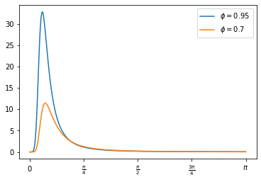
Figure 1: Spectrum Associated with HP filtering an AR(1)
Another way to see this is look at the autocovariance function of the implied process, which we can recover by the inverse fourier transform as discussed in class:
\begin{eqnarray} \gamma_k = \int_{-\pi}^{\pi} f^{Y}(\omega)e^{i\omega k}. \end{eqnarray}
The HP filter induces complex dynamics into the process!
from scipy.integrate import quad
H = 20
really_small = 1e-8
acf = [quad(lambda omega:
                 2*f(omega)*np.cos(omega*k), really_small, np.pi)[0]
            for k in np.arange(H)]
plt.plot(acf)

phi = 0.95
acf = [ phi**j / (1-phi**2) for j in np.arange(H)]
plt.plot(acf, linestyle='dashed')
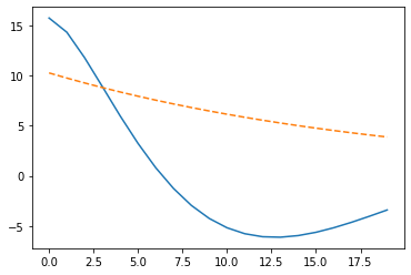
Figure 2: ACF of AR(1) vs. ACF of HP filtered Component