Stock and Watson (2007) in pymc3 and Stan
This file is available as Jupyter Notebook.
The STOCK_2007 model inflation as an unobserved components models:
\begin{eqnarray} \pi_t &=& \tau_t + \eta_t \\\ \tau_t &=& \tau_{t-1} + \epsilon_t \end{eqnarray}
where \(\eta_t\) and \(\epsilon_t\) are independently and identically distributed with mean 0 and variances \(\sigma_\eta^2\) and \(\sigma_\epsilon^2\).
A Replication
First we start by importing some standard libraries.
%matplotlib inline
import matplotlib.pyplot as plt
import numpy as np
import pandas as p
Next we get the data used and plot it.
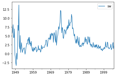
Figure 1: Inflation Data
from pymc3 import Model, Normal, InverseGamma, sample
from pymc3.distributions.timeseries import GaussianRandomWalk

from pymc3 import Uniform, Deterministic
from pymc3.math import exp, sqrt

y = sw_infl['1953':'2004'].values.flatten()

with Model() as ucsv_model:

    gamma = 0.2
    ln_sigma2_eps = GaussianRandomWalk('ln_sigma2_eps', sd=gamma, shape=len(y)-1)
    ln_sigma2_eta = GaussianRandomWalk('ln_sigma2_eta', sd=gamma, shape=len(y))

    sigma_eps = Deterministic('sigma_eps', exp(0.5*ln_sigma2_eps))
    tau = GaussianRandomWalk('tau', sd=sigma_eps, shape=len(y))

    sigma_eta = Deterministic('sigma_eta', exp(0.5*ln_sigma2_eta))
    pinf = Normal('pi',mu=tau, sd=sigma_eta, observed=y)

    temp = Deterministic('temp', sigma_eta[1:]**2/(sigma_eps**2 + 2*sigma_eta[1:]**2))
    theta = Deterministic('theta', (-1 + sqrt(1-4*temp*temp)) /(-2*temp))
with ucsv_model:
    trace = sample(2000)

sigma_eps_df = p.DataFrame(trace['sigma_eps'],columns=sw_infl['1953Q2':'2004'].index)
sigma_eta_df = p.DataFrame(trace['sigma_eta'],columns=sw_infl['1953':'2004'].index)
theta_df = p.DataFrame(trace['theta'],columns=sw_infl['1953Q2':'2004'].index)
def sw_figure2(sigma_eps, sigma_eta, theta):
    fig,ax = plt.subplots(nrows=3, sharex=True)

    for i, para in enumerate([sigma_eps, sigma_eta, theta]):

        if i < 2:
            ylim = (0,2)
        else:
            ylim = (0,1)

        para.median().plot(ax=ax[i], color='black', ylim=ylim)
        para.quantile([0.16,0.84]).T.plot(ax=ax[i], color='black',
                                          linestyle='dashed', legend=False)

    plt.tight_layout()
    fig.set_size_inches(3,9)

sw_figure2(sigma_eps_df, sigma_eta_df, theta_df)
NameErrorTraceback (most recent call last)
<ipython-input-8-16860f4ca04e> in <module>
     16     fig.set_size_inches(3,9)
     17
---> 18 sw_figure2(sigma_eps_df, sigma_eta_df, theta_df)

NameError: name 'sigma_eps_df' is not defined
Bibliography
[STOCK_2007] Stock & Watson, Why Has U.S. Inflation Become Harder to Forecast?, Journal of Money, Credit and Banking, 39, 3 33 (2007). link. doi. ↩