ECON 616: Machine Learning
Intro + Defintions
Background
- Stuff written by economists: Varian (2014),
Mullainathan and Spiess (2017), Athey (2018)
- Useful books: Hastie, Tibshirani, and Friedman (2009),
- Gentle introduction: Machine Learning on http://coursera.org;
many other things on the internet (of varying quality).
- Computation:
scikit-learn(python).
“Machine Learning” definition
Hard to define; context dependent;
… a field that develops algorithms designed to applied to datasets with the main areas of focus being prediction (regression), classification, and clustering or grouping tasks.
Broadly speaking, two branches:
- Supervised: dependent variables known (think predicting output growth)
- Unsupervised: dependent variables unknown (think classifying recessions)
A Dictionary
| Econometrics | ML | |
|---|---|---|
| \(\underbrace{y}_{T\times 1} = \{y_{1:T}\}\) | Endogenous | outcome |
| \(\underbrace{X}_{T\times n} = \{x_{1:T}\}\) | Exogenous | Feature |
| \(1:T\) | “in sample” | “training” |
| \(T:T+V \) | ??? not enough data! | “validation” |
| \(T+V:T+V+O\) | “out of sample” | “testing” |
Today I’ll concentrate on prediction (regression) problems.
\[
\hat y = f(X;\theta)
\]
Economists would call this modeling the conditional expectation,
MLers the hypothesis function.
It all starts with a loss funciton
Generally speaking, we can write (any) estimation problem as
essentially a loss minizimation problem.
Let \(L\)
\[
L(\hat y, y) = L(f(X;\theta), y)
\]
Be a loss function (sometimes called a “cost” function).
Estimation in ML: pick \(\theta\) to minimize loss.
ML more concerned with minimizing my loss than inference on
\(\theta\) per se.
Forget standard errors…
Gradient Descent
- In practice, it is often not possible to minimize the loss
function analytically.
- In fact, most machine learning models correspond to functions
\(f(\cdot;\theta)\) that are highly nonlinear in \(\theta\).
- In addition to an explosition of datasets, a large part of the
success of machine learning algorithms is the development of
robust minimization routines.
- The first one everyone learns is called
gradient descent: \[ \theta ’ = \theta + \alpha \frac{d L(\hat y,y)}{d \theta} \] - You can use this for OLS when \(N > T\).
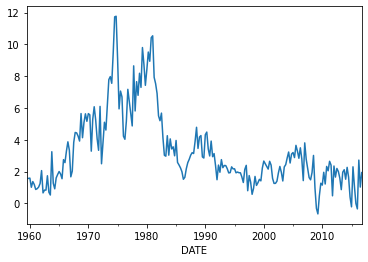
Example: Forecasting Inflation
Let’s consider forecasting (GDP deflator) inflation.
Linear Regression
- Consider forecasting inflation using only it’s lag and constant.
- Training sample: 1985-2000
- Testing sample: 2001-2015
- scikit-learn code
from sklearn.linear_model import LinearRegression
linear_model_univariate = LinearRegression()

train_start, train_end = '1985', '2000'
inf['inf_L1'] = inf.GDPDEF.shift(1)
inf = inf.dropna(how='any')
inftrain = inf[train_start:train_end]
Xtrain,ytrain = (inftrain.inf_L1.values.reshape(-1,1),
                 inftrain.inf)
fitted_ols = linear_model_univariate.fit(Xtrain,ytrain)
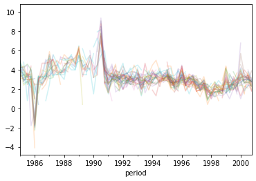
Many regressors
Let’s add the individual spf forecasts to our regression.
/home/eherbst/miniconda3/lib/python3.8/site-packages/openpyxl/worksheet/header_footer.py:48: UserWarning: Cannot parse header or footer so it will be ignored
  warn("""Cannot parse header or footer so it will be ignored""")
Estimating this in scikit learn is easy
spf_flatted_zero = spf_flat.fillna(0.)

spfX = spf_flatted_zero[train_forecasters][train_start:train_end]
spfXtrain = np.c_[Xtrain, spfX]

linear_model_spf = LinearRegression()
fitted_ols_spf = linear_model_spf.fit(spfXtrain,ytrain)
| Train | Test | |
|---|---|---|
| LS-univariate | 0.59 | 2.28 |
| LS-SPF | 0 | 2.1 |
Regularization
We’ve got way too many variables – our model does horrible out of
sample!
Their are many regularization techniques available for variable selection
Conventional: AIC, BIC
Alternative approach: Penalized regression.
Consider the loss function:
\[
L(\hat y,y) = \frac{1}{2T} \sum_{t=1}^T (f(x_t;\theta) - y)^2 +
\lambda \sum_{i=1}^N \left[(1-\alpha)|\theta_i| + \alpha|\theta_i|^2\right].
\]
This is called elastic net regression. When \(\lambda = 0\), we’re back to OLS.
Many special cases.
Ridge Regression
The ridge regression Hoerl and Kennard (2004) is special case where \(\alpha
= 1\).
Long (1940s) used in statistics and econometrics.
This is sometimes called (or is a special case of) “Tikhonov regularization”
It’s an L2 penalty, so it’s won’t force parameters to be exactly
zero.
Can be formulatd as Bayesian linear regression.
from sklearn.linear_model import Ridge
fitted_ridge = Ridge().fit(spfXtrain,ytrain)
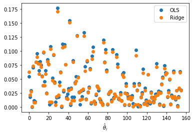
LS vs Ridge (\(\lambda = 1\)) Coefficients
Lasso Regression
Set \(\alpha = 0\)
- This is an \(L1\) penalty – forces small coefficients to exactly 0.
- Greatly reduces model complexity.
- Can you give economic interpretation to the parameters?
- Bayesian interpetation: Laplace prior in \(\theta\).
from sklearn.linear_model import Lasso
fitted_lasso = Lasso().fit(spfXtrain,ytrain)
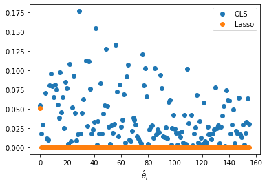
LS vs Lasso (\(\lambda = 1\)) Coefficients
Picking \(\lambda\)
Use “rule of thumb” given subject matter.
Tradition validation: Use many \(\lambda\) on your test sample, Assess accuracy of each on validation sample, pick one which gives minimum loss.
Cross validation:
- Divide sample in \(K\) parts:
- For each \(k \in K\), pick \(\lambda_k\), fit model using the \(K-k\) sample.
- Plot Loss against \(\lambda_k\), pick \(\lambda\) which yields minimum.
Chernozhukov et al. (2018) derive “Oracle” properties for LASSO, pick \(\lambda\) based on this.
| Method | Train | Train |
|---|---|---|
| Least Squares (Univariate) | 0.35 | 0.71 |
| Least Squares (SPF) | 0.0 | 0.68 |
| Least Squares (SPF-Ridge) | 0.0003 | 0.67 |
| Least Squares (SPF-Lasso) | 0.59 | 0.96 |
Support Vector Machines
Support Vector Machines
- While Elastic net, lasso, and ridge were designed around regularization, other machine learning techniques are designed to fit more flexible models.
- Support Vector Machines are typically used in classification
problems.
- Essentially SVM constructs a seperating hyperplane (hello 2nd
basic welfare theorem), to optimally seperate (“classify”)
points.
- What’s cool about the support vector machine is that you can use
a kernel trick, so your hyperplanes need not correspond to lines
in euclidean space.
- For regression, the hyperplane will be prediction.
Support Vector Machines
- Explicit form: \[ f(x;\theta) = \sum_{i=1}^n \theta_i h(x) + \theta_0. \]
- \(\epsilon\) insensitive loss: function does not penalize
predictions which are in an \(\epsilon\) of the, otherwise the
penalized by a factor relatid to \(C\) (comes from dual problem).
- Key choice here: the choice of kernel
- \(\epsilon\), \(C\) chosen by (cross) validation.
Estimating Support Vector Machine
from sklearn.svm import SVR
fitted_svm = SVR().fit(Xtrain,ytrain)
| Method | Train | Train |
|---|---|---|
| Least Squares (Univariate) | 0.35 | 0.71 |
| Least Squares (SVM) | 0.06 | 0.73 |
Other ML Techniques
Other Popular ML Techniques
Forests: partition feature space, fit individual models condition on subsample.
Obviously, you can partition ad infinitum to obtain perfect predictions.
Random forest: pick random subspace/set; average over these random models.
Long literature in econometrics about model averaging Bates and Granger (1969).
Further refinements: bagging, boosting.
Neural Networks
Neural Networks
Let’s construct a hypothesis function using a neural network.
Suppose that we have \(N\) features in \(x_t\).
(Let \(x_{0,t}\) be the intercept.)
Neural Networks are modeled after the way neurons work in a brain as basical
computational units.
- Inputs (dendrites) channeled to outputs (axons)
- Here the input is \(x_t\) and the output is \(f(x_t;\theta)\).
- The neuron maps the inputs to outputs using a (nonlinear) activation function \(\(g\)\).
- By adding layers of neurons, we can create very (arbitrary) complex prediction models (all “logical gates”).
Neural Networks, continued
Drop the \(t\) subscript. Consider: \[ \left[\begin{array}{c} x_{0} \\ \vdots \\ x_{N} \end{array}\right] \rightarrow [~] \rightarrow f(x;\theta) \] \(a_i^j\) activation of unit \(i\) in layer \(j\).
\(\beta^j\) matrix of weights controlling function mapping layer \(j\) to layer \(j+1\). \[ \left[\begin{array}{c} x_{0} \\ \vdots \\ x_{N} \end{array}\right] \rightarrow \left[\begin{array}{c} a_{0}^2 \\ \vdots \\ a_{N}^2 \end{array}\right] \rightarrow f(x;\theta) \].
Neural Networks in a figure
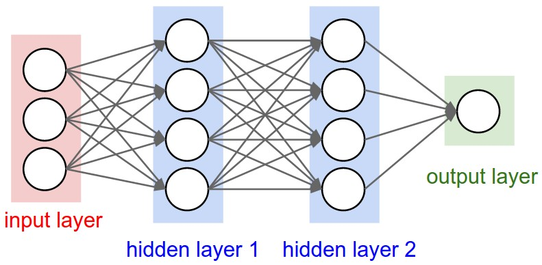
Neural Networks Continued
If \(N = 2\) and our neural network has \(1\) hidden layer.
\begin{eqnarray} a_1^2 &=& g(\theta_{10}^1 x_0 + \theta_{11}^1 x_1 + \theta_{12}^1 x_2) \nonumber \\ a_2^2 &=& g(\theta_{20}^1 x_0 + \theta_{21}^1 x_1 + \theta_{22}^1 x_2) \nonumber \\ f(x;\theta) &=& g(\theta_{10}^2 a_0^2 + \theta_{11}^2 a_1^2 + \theta_{12}^2 a_2^2 \\ \end{eqnarray}
(\(a_0^j\) is always a constant (“bias”) by convention.)
Matrix of coefficients \(\theta^j\) sometimes called weights
Depending on \(g\), \(f\) is highly nonlinear in \(x\)! Good and bad …
Which activation function?
| name | |
|---|---|
| linear | \(\theta x\) |
| sigmoid | \(1/(1+e^{-\theta x}\) |
| tanh | \(tanh(\theta x)\) |
| rectified linear unit | \(max(0,\theta x)\) |
| … | … |
How to pick \(g\)…?
- Dependent on problem: prediction vs classification.
- Think about derivate of cost/loss wrt deep parameters.
- Trial and error
How to estimate this model.
Just like any other ML model: minimize the loss!
Gradient descent needs a derivative
back propagation algorithm
Application: Nakamura (2005)
- Nakamura (2005) considers (GDP deflator) inflation forecasting
with a neural network.
- Model has 1 hidden layer, and uses a hyperbolic tangent
activation function
- Can be explicitly written as:
\[
\hat\pi_{t+h} = w_{2,1}\tanh(w_{1,1}’ x_{t} + b_{1,1}) + w_{2,2}\tanh(w_{1,2}'
x_{t} + b_{1,2}) + b_{2,1}
\]
- \(x_{t}\) is a vector of \(t-1\) variables. For simplicity, I’ll consider \(x_{t-1} = \pi_{t-1}\).
scikit-learn code
from sklearn.neural_network import MLPRegressor

NN = MLPRegressor(hidden_layer_sizes=(2,),
                  activation='tanh',
                  alpha=1e-6,
                  max_iter=10000,
                  solver='lbfgs')

fitted_NN = NN.fit(Xtrain,ytrain)
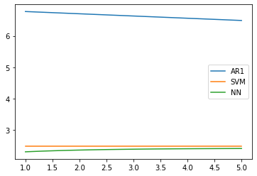
Neural Network vs. AR(1): Predicted Values
What is the “right” method to use
You might have guessed…
Wolpert and Macready (1997): A universal learning algorithm does cannot exist.
Need prior knowledge about problem…
This is has been present in econometrics for a very long time…
There’s no free lunch!.