ECON 616: Lecture 1: Time Series Basics
Lecture 1: Time Series Basics
References
Overview: Chapters 1-3 from (James Hamilton, 1994).
Technical Details: Chapters 2-3 from (Brockwell, Peter J. and Davis, Richard A., 1987).
Intuition: Chapters 1-4 from (John Cochrane, 2005).
Time Series
A time series is a family of random variables indexed by time
\(\{Y_t, t\in T\}\) defined on a probability space \((\Omega, \mathcal
F, P)\).
(Everybody uses “time series” to mean both the random variables and their realizations)
For this class, \(T = \left\{0, \pm 1, \pm 2, \ldots\right\}\).
Some examples:
- \(y_t = \beta_0 + \beta_1 t + \epsilon_t, \quad \epsilon_t \sim iid N(0, \sigma^2)\).
- \(y_t = \rho y_{t-1} + \epsilon_t, \quad \epsilon_t \sim iid N(0, \sigma^2)\).
- \(y_t = \epsilon_1 \cos(\omega t) + \epsilon_2 \sin (\omega t), \quad \omega \in [0, 2\pi)\).
Time Series – Examples
Why time series analysis?
Seems like any area of econometrics, but:
We (often) only have one realization for a given time series probability model (and it’s short)!
(A single path of 282 quarterly observations for real GDP since 1948…)
Focus (mostly) on parametric models to describe time series.
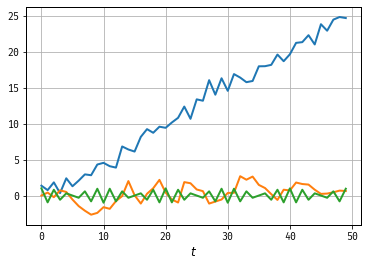
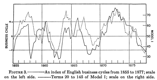
(A long time ago, economists noticed that time series statistical models could mimic the properties of economic data.)
More emphasis on prediction than some subfields.
(Eugen Slutzky, 1937)
Definitions
The autocovariance function of a time series is the set of functions \(\{\gamma_t(\tau), t\in T\}\)
\[
\gamma_t(\tau) = \mathbb E\left[ (Y_t - \mathbb EY_t) (Y_{t+\tau} - \mathbb EY_{t+\tau})’\right]
\]
A time series is covariance stationary if
- \(E\left[Y_t^2\right] = \sigma^2 < \infty\) for all \(t\in T\).
- \(E\left[Y_t\right]=\mu\) for all \(t\in T\).
- \(\gamma_t(\tau) = \gamma(\tau)\) for all \(t,\tau \in T\).
Note that \(|\gamma(\tau)| \le \gamma(0)\) and \(\gamma(\tau) = \gamma(-\tau)\).
Some Examples
- \(y_t = \beta t + \epsilon_t, \epsilon\sim iid N(0,\sigma^2)\). \(\mathbb E[y_t] = \beta t\), depends on time, not covariance stationary!
- \(y_t = \epsilon_t + 0.5\epsilon_{t-1}, \epsilon\sim iid N(0,\sigma^2)\) \(\mathbb E[y_t] = 0, \quad \gamma(0) = 1.25\sigma^2, \quad \gamma(\pm 1) = 0.5\sigma^2, \quad \gamma(\tau) = 0\) \(\implies\) covariance stationary.
Building Blocks of Stationary Processes
A stationary process \(\{Z_t\}\) is called white noise if it satisfies
- \(E[Z_t] = 0\).
- \(\gamma(0) = \sigma^2\).
- \(\gamma(\tau) = 0\) for \(\tau \ne 0\).
These processes are kind of boring on their own, but using them we can construct arbitrary stationary processes!
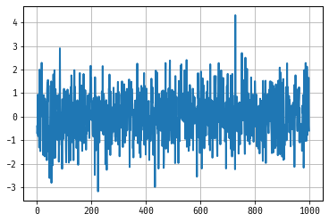
Special Case: \(Z_t \sim iid N(0, \sigma^2)\)
White Noise
Asymptotics for Covariance Stationary MA pr.
Covariance Stationarity isn’t necessary or sufficient to ensure the convergence of sample averages to population averages.
We’ll talk about a special case now.
Consider the moving average process of order \(q\)
\[
y_t = \epsilon_t + \theta_1 \epsilon_{t-1} + \ldots + \theta_q \epsilon_{t-q}
\]
where \(\epsilon_t\) is iid \(WN(0,\sigma^2)\).
We’ll show a weak law of large numbers and central limit theorem applies to this process using the Beveridge-Nelson decomposition following Phillips and Solo (1992).
Using the lag operator \(LX_t = X_{t-1}\) we can write
\[
y_t = \theta(L)\epsilon_t, \quad \theta(z) = 1 + \theta_1 z + \ldots + \theta_q z^q.
\]
Deriving Asymptotics
Write \(\theta(\cdot)\) in Taylor expansion-ish sort of way
\begin{eqnarray} \theta(L) &=& \sum_{j=0}^q \theta_j L^j, \nonumber \\ &=& \left(\sum_{j=0}^q \theta_j - \sum_{j=1}^q \theta_j\right) + \left(\sum_{j=1}^q \theta_j - \sum_{j=2}^q \theta_j\right)L \nonumber \\ &~&+ \left(\sum_{j=2}^q \theta_j - \sum_{j=3}^q \theta_j\right)L^2 + \ldots \nonumber \\ &=& \sum_{j=0}^q \theta_j + \left(\sum_{j=1}^q\theta_j\right)(L-1) + \left(\sum_{j=2}^q\theta_j\right)(L^2-L) + \ldots\nonumber\\ &=& \theta(1) + \hat\theta_1(L-1) + \hat\theta_2 L (L-1) + \ldots \nonumber\\ &=& \theta(1) + \hat\theta(L)(L-1) \nonumber \end{eqnarray}
WLLN / CLT
We can write \(y_t\) as \[ y_t = \theta(1) \epsilon_t + \hat\theta(L)\epsilon_{t-1} - \hat\theta(L)\epsilon_{t} \] An average of \(y_t\) cancels most of the second and third term … \[ \frac1T \sum_{t=1}^T y_t = \frac{1}{T}\theta(1) \sum_{t=1}^T \epsilon_t + \frac1T\left(\hat\theta(L)\epsilon_0 - \hat\theta(L)\epsilon_T\right) \] We have \[ \frac{1}{\sqrt{T}}\left(\hat\theta(L)\epsilon_0 - \hat\theta(L)\epsilon_T\right) \rightarrow 0. \] Then we can apply a WLLN / CLT for iid sequences with Slutzky’s Theorem to deduce that \[ \frac1T \sum_{t=1}^T y_t \rightarrow 0 \mbox{ and } \frac{1}{\sqrt{T}}\sum_{t=1}^T y_t \rightarrow N(0, \sigma^2 \theta(1)^2) \]
ARMA Processes
ARMA Processes
The processes \(\{Y_t\}\) is said to be an ARMA\((p,q)\) process if \(\{Y_t\}\) is stationary and if it can be represented by the linear difference equation:
\[ Y_t = \phi_1 Y_{t-1} + \ldots \phi_p Y_{t-p} + Z_t + \theta_1 Z_{t-1} + \ldots + \theta_q Z_{t-q} \] with \(\{Z_t\} \sim WN(0,\sigma^2)\). Using the lag operator \(LX_t = X_{t-1}\) we can write: \[ \phi(L)Y_t = \theta(L)Z_t \] where \[ \phi(z) = 1 - \phi_1 z - \ldots \phi_p z^p \mbox{ and } \theta(z) = 1 + \theta_1 z + \ldots + \theta_q z^q. \] Special cases:
- \(AR(1) : Y_t = \phi_1 Y_{t-1} + Z_t\).
- \(MA(1) : Y_t = Z_t + \theta_1 Z_{t-1}\).
- \(AR(p)\), \(MA(q)\), \(\ldots\)
Why are ARMA processes important?
- Defined in terms of linear difference equations (something we know a lot about!)
- Parametric family \(\implies\) some hope for estimating these things
- It turns out that for any stationary process with autocovariance function \(\gamma_Y(\cdot)\) with \(\lim_{\tau\rightarrow\infty}\gamma(\tau) = 0\), we can, for any integer \(k>0\), find an ARMA process with \(\gamma(\tau) = \gamma_Y(\tau)\) for \(\tau = 0, 1, \ldots, k\).
They are pretty flexible!
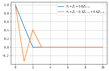
MA(q) Process Revisited
\[ Y_t = Z_t + \theta_1 Z_{t-1} + \ldots + \theta_q Z_{t-q} \] Is it covariance stationary? Well, \[ \mathbb E[Y_t] = \mathbb E[Z_t] + \theta_1 \mathbb E[Z_{t-1}] + \ldots + \theta_q \mathbb E[ Z_{t-q}] = 0 \] and \(\mathbb E[Y_t Y_{t-h} ] =\) \[ \mathbb E[( Z_t + \theta_1 Z_{t-1} + \ldots + \theta_q Z_{t-q}) ( Z_{t-h} + \theta_1 Z_{t-h-1} + \ldots + \theta_q Z_{t-h-q})] \]
If \(q\le h\), this equals \(\sigma^2(\theta_h\theta_0 + \ldots +\theta_q\theta_{q-h})\) and 0 otherwise.
This doesn’t depend on \(t\), so this process is covariance stationary regardless of values of \(\theta\).
Autocorrelation Function
AR(1) Model
\[ Y_t = \phi_1 Y_{t-1} + Z_t \] From the perspective of a linear difference equation, \(Y_t\) can be solved for as a function \(\{Z_t\}\) via backwards subsitution:
\begin{eqnarray} Y_t &=& \phi_1(\phi_1 Y_{t-2} + Z_{t-1}) + Z_{t}\\ &=& Z_t + \phi_1 Z_{t-1} + \phi_1^2 Z_{t-2} +\ldots \\ &=& \sum_{j=0}^{\infty} \phi_1^j Z_{t-j} \end{eqnarray}
How do we know whether this is covariance stationary?
Analysis of AR(1), continued
We want to know if \(Y_t\) converges to some random variable as we consider the infinite past of innovations.
The relevant concept (assuming that \(E[Y_t^2] < \infty\)) is mean square convergence. We say that \(Y_t\) converges in mean square to a random variable \(Y\) if
\[
\mathbb E\left[(Y_t - Y)^2\right] \longrightarrow 0 \mbox{ as } t\longrightarrow \infty.
\]
It turns out that there is a connection to deterministic sums \(\sum_{j=0}^\infty a_j\).
We can prove mean square convergence by showing that the sequence generated by partial summations satisfies a Cauchy criteria, very similar to the way you would for a deterministic sequence.
Analysis of AR(1), continued
What this boils down to: We need square summability: \(\sum_{j=0}^{\infty} (\phi_1^j)^2 < \infty\).
We’ll often work with the stronger condition absolute summability : \(\sum_{j=0}^{\infty} |\phi_1^j| < \infty\).
For the AR(1) model, this means we need \(|\phi_1| < 1\), for covariance stationarity.
Relationship Between AR and MA Processes
You may have noticed that we worked with the infinite moving average representation of the AR(1) model to show convergence. We got there by doing some lag operator arithmetic:
\[
(1-\phi_1L)Y_t = Z_t
\]
We inverted the polynomial \(\phi(z) = (1-\phi_1 z)\) by
\[
(1-\phi_1z)^{-1} = 1 + \phi_1 z + \phi_1^2 z^2 + \ldots
\]
Note that this is only valid when \(|\phi_1 z|<1 \implies\) we can’t always perform inversion!
To think about covariance stationarity in the context of ARMA processes, we always try to use the \(MA(\infty)\) representation of a given series.
A General Theorem
If \(\{X_t\}\) is a covariance stationary process with autocovariance function \(\gamma_X(\cdot)\) and if \(\sum_{j=0}^\infty |\theta_j| < \infty\), than the infinite sum \[ Y_t = \theta(L)X_t = \sum_{j=0}^\infty \theta_j X_{t-j} \] converges in mean square. The process \(\{Y_t\}\) is covariance stationary with autocovariance function \[ \gamma(h) = \sum_{j=0}^\infty\sum_{k=0}^\infty \theta_j\theta_k \gamma_x(h-j+k) \] If the autocovariances of \(\{X_t\}\) are absolutely summable, then so are the autocovrainces of \(\{Y_t\}\).
Back to AR(1)
\[ Y_t = \phi_1 Y_{t-1} + Z_t, \quad Z_t \sim WN(0,\sigma^2),\quad |\phi_1|<1 \] The variance can be found using the MA(∞) representation
\begin{eqnarray} Y_t = \sum_{j=0}^\infty \phi_1^j Z_{t-j} &\implies& \nonumber \\ \mathbb E[Y_t^2] &=& \mathbb E \left[\left(\sum_{j=0}^\infty \phi_1^j Z_{t-j} \right) \left(\sum_{j=0}^\infty \phi_1^j Z_{t-j}\right) \right] \nonumber \\ &=& \sum_{j=0}^\infty\mathbb E \left[\phi_1^{2j} Z_{t-j}^2\right] = \sum_{j=0}^\infty\phi_1^{2j} \sigma^2 \end{eqnarray}
This means that \[ \gamma(0) = \mathbb V[Y_t] = \frac{\sigma^2}{1-\phi_1^2} \]
Autocovariance of AR(1)
To find the autocovariance:
\[
Y_t Y_{t-1} = \phi_1 Y_{t-1}^2 + Z_t Y_{t-1} \implies \gamma(1) = \phi_1 \gamma(0)
\]
\[
Y_t Y_{t-2} = \phi_1 Y_{t-1}Y_{t-2} + Z_t Y_{t-2} \implies \gamma(2) = \phi_1 \gamma(1)
\]
\[
Y_t Y_{t-3} = \phi_1 Y_{t-1}Y_{t-3} + Z_t Y_{t-3} \implies \gamma(3) = \phi_1 \gamma(2)
\]
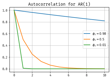
Let’s look at autocorrelation
\[
\rho(\tau) = \frac{\gamma(\tau)}{\gamma(0)}
\]
Autocorrelation for AR(1)
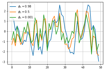
Simulated Paths
Analysis of AR(2) Model
\[ Y_t = \phi_1 Y_{t-1} + \phi_2 Y_{t-2} + \epsilon_t \] Which means \[ \phi(L) Y_t = \epsilon_t, \quad \phi(z) = 1 - \phi_1 z - \phi_2 z^2 \] Under what conditions can we invert \(\phi(\cdot)\)? Factoring the polynomial \[ 1 - \phi_1 z - \phi_2 z^2 = (1-\lambda_1 z) (1-\lambda_2 z) \] Using the above theorem, if both \(|\lambda_1|\) and \(|\lambda_2|\) are less than one in length (they can be complex!) we can apply the earlier logic succesively to obtain conditions for covariance stationarity.
Note: \(\lambda_1\lambda_2 = -\phi_2\) and \(\lambda_1 + \lambda_2 = \phi_1\)
Companion Form
\begin{eqnarray}\left[\begin{array}{c}Y_t \\ Y_{t-1} \end{array}\right] = \left[\begin{array}{cc}\phi_1 & \phi_2 \\ 1 & 0 \end{array}\right] \left[\begin{array}{c}Y_{t-1} \\ Y_{t-2} \end{array}\right] + \left[\begin{array}{c}\epsilon_t\\ 0 \end{array}\right]\end{eqnarray}
\({\mathbf Y}_t = F {\mathbf Y}_{t-1} + {\mathbf \epsilon_t}\)
\(F\) has eigenvalues \(\lambda\) which solve \(\lambda^2 - \phi_1 \lambda - \phi_2 = 0\)
Finding the Autocovariance Function
Multiplying and using the symmetry of the autocovariance function:
\begin{eqnarray} Y_t &:&\gamma(0) = \phi_1\gamma(1) + \phi_2\gamma(2) + \sigma^2 \\ Y_{t-1} &:& \gamma(1) = \phi_1\gamma(0) + \phi_2\gamma(1) \\ Y_{t-2} &:& \gamma(2) = \phi_1\gamma(1) + \phi_2\gamma(0) \\ &\vdots& \\ Y_{t-h} &:& \gamma(h) = \phi_1\gamma(h-1) + \phi_2\gamma(h-2) \end{eqnarray}
We can solve for \(\gamma(0), \gamma(1), \gamma(2)\) using the first three equations: \[ \gamma(0) = \frac{(1-\phi_2)\sigma^2}{(1+\phi_2)[(1-\phi_2)^2 - \phi_1^2]} \] We can solve for the rest using the recursions.
Note pth order AR(1) have autocovariances / autocorrelations that follow the same pth order difference equations.
Autocorrelations: call these Yule-Walker equations.
Why are we so obsessed with autocovariance/correlation functions?
- For covariance stationary processes, we are really only concerned with the first two moments.
- If, in addition, the white noise is actually IID normal, those two moments characterize everything!
- So if two processes have the same autocovariance (and mean…), they’re the same.
- We saw that with the \(AR(1)\) and \(MA(\infty)\) example.
- How do we distinguish between the different processes yielding an identical series?
Invertibility
Recall
\[
\phi(L) Y_t = \theta(L) \epsilon_t
\]
We already discussed conditions under which we can invert \(\phi(L)\) for the AR(1) model to represent \(Y_t\) as an \(MA(\infty)\).
What about other direction? An MA process is invertible if \(\theta(L)^{-1}\) exists.
so \(MA(1) : |\theta_1|<1, \quad MA(q): \ldots\)
MA(1) with \(|\theta_1| > 1\)
Consider
\[
Y_t = \epsilon_t + 0.5\epsilon_{t-1}, \quad \epsilon_t \sim WN(0, \sigma^2)
\]
\(\gamma(0) = 1.25\sigma^2, \quad \gamma(1) = 0.5\sigma^2\).
vs.
\[
Y_t = \tilde\epsilon_t + 2\tilde\epsilon_{t-1}, \quad \epsilon_t \sim WN(0, \tilde\sigma^2)
\]
\(\gamma(0) = 5\tilde\sigma^2, \quad \gamma(1) = 2\tilde\sigma^2\)
For \(\sigma = 2\tilde\sigma\), these are the same!
Prefer invertible process:
- Mimics AR case.
- Intuitive to think of errors as decaying.
- Noninvertibility pops up in macro: news shocks!
Why ARMA, again?
ARMA models seem cool, but they are inherently linear
Many important phenomenom are nonlinear (hello great recession!)
It turns out that any covariance stationary process has a linear ARMA representation!
This is called the Wold Theorem; it’s a big deal.
Wold Decomposition
Theorem Any zero mean covariance stationary process \(\{Y_t\}\) can be represented as \[ Y_t = \sum_{j=0}^\infty \psi_j \epsilon_{t-j} + \kappa_t \] where \(\psi_0=1\) and \(\sum_{j=0}^\infty \psi_j^2 < \infty\). The term \(\epsilon_t\) is white noise are represents the error made in forecasting \(Y_t\) on the basis of a linear function of lagged \(Y\) (denoted by \(\hat {\mathbb E}[\cdot|\cdot]\)): \[ \epsilon_t = y_t - \hat {\mathbb E}[Y_t|y_{t-1}, y_{t-2},\cdot] \] The value of \(\kappa_t\) is uncorrelated with \(\epsilon_{t-j}\) for any value of \(j\), and can be predicted arbitrary well from a linear function of past values of \(Y\): \[ \kappa_t = \hat {\mathbb E}[\kappa_t|y_{t-1}, y_{t-2},\cdot] \]
More Large Sample Stuff
Strict Stationarity
A time series is strictly stationary if for all \(t_1,\ldots,t_k, k, h \in T\) if
\(Y_{t_1}, \ldots, Y_{t_k} \sim Y_{t_1+h}, \ldots, Y_{t_k+h}\)
What is the relationship between strict and covariance stationarity?
\(\{Y_t\}\) strictly stationary (with finite second moment) \(\implies\) covariance stationarity.
The corollary need not be true!
Important Exception if \(\{Y_t\}\) is gaussian series covariance stationarity \(\implies\) strict stationarity.
Ergodicity
In earlier econometrics classes, you (might have) examined large sample properties of estimators using LLN and CLT for sums of independent RVs.
Times series are obviously not independent, so we need some other tools. Under what conditions do time averages converge to population averages. One helpful concept:
A stationary process is said to be ergodic if, for any two bounded and measurable functions \(f: \mathbb R^k \longrightarrow \mathbb R\) and \(g : {\mathbb R}^l \longrightarrow \mathbb R\),
\begin{eqnarray} \lim_{n\rightarrow\infty} \left|\mathbb{E} \left[ f(y_t,\ldots,y_{t+k})g(y_{t+n},\ldots,g_{t+n+l}\right]\right| \nonumber \- \left|\mathbb{E} \left[ f(y_t,\ldots,y_{t+k})\right]\right| \left|\mathbb{E}\left[g(y_{t+n},\ldots,y_{t+n+l}\right]\right| = 0 \nonumber \end{eqnarray}
Ergodicity is a tedious concept. At an intuitive level, a process if ergodic if the dependence between an event today and event at some horizon in the future vanishes as the horizon increases.
The Ergodic Theorem
If \(\{y_t\}\) is strictly stationary and ergodic with \(\mathbb E[y_1] < \infty\), then \[ \frac1T \sum_{t=1}^T y_t\longrightarrow E[y_1] \]
CLT for strictly stationary and ergodic processes_
If \(\{y_t\}\) is strictly stationary and ergodic with \(\mathbb E[y_1] < \infty\), \(E[y_1^2] < \infty\), and \(\bar\sigma^2 = var(T^{-1/2} \sum y_t) \rightarrow \bar\sigma^2 < \infty\), then \[ \frac{1}{\sqrt{T}\bar\sigma_T}\sum_{t=1}^T y_t \rightarrow N(0,1) \]
Facts About Ergodic Theorem
- iid sequences are stationary and ergodic
- If \(\{Y_t\}\) is strictly stationary and ergodic, and \(f: \mathbb R^\infty \rightarrow \mathbb R\) is a measurable function:
\[ Z_t = f(\{Y_t\}) \] Then \(Z_t\) is strictly stationary and ergodic.
(Note this is for strictly stationary processes!)
Example
Example: an \(MA(\infty)\) with iid Gaussian white noise. \[ Y_t = \sum_{j=0}^\infty \theta_j\epsilon_{t-j}, \quad \sum_{j=0}^\infty| \theta_j| < \infty. \] This means that \(\{Y_t\}, \{Y_t^2\}, \mbox { and } \{Y_tY_{t-h}\}\) are ergodic! \[ \frac1T \sum_{t=0}^\infty Y_t \rightarrow \mathbb E[Y_0], \quad \frac1T \sum_{t=0}^\infty Y_t^2 \rightarrow \mathbb E[Y_0^2], \quad \] \[ \frac1T \sum_{t=0}^\infty Y_tY_{t-h} \rightarrow \mathbb E[Y_0Y_{-h}], \]
Martingale Difference Sequences
\(\{Z_t \}\) is a Martingale Difference Sequence (with respect to the information sets \(\{ {\cal F}_t \}\)) if \[ E[Z_t|{\cal F}_{t-1}] = 0 \quad \mbox{for all} \;\; t \] LLN and CLT for MDS Let \(\{Y_t, {\cal F}_t\}\) be a martingale difference sequence such that \(E[|Y_t|^{2r}] < \Delta < \infty\) for some \(r > 1\), and all \(t\).
- Then \(\bar{Y}_T = T^{-1} \sum_{t=1}^T Y_t \stackrel{p}{\longrightarrow} 0\).
- Moreover, if \(var(\sqrt{T} \bar{Y}_T) = \bar{\sigma}_T^2 \rightarrow \sigma^2 > 0\), then \(\sqrt{T} \bar{Y}_T / \bar{\sigma}_T \Longrightarrow {\cal N}(0,1)\). \(\Box\)
An Example of an MDS
An investor faces a choice between a stock which generates real
return \(r_t\), and a nominal bond with guaranteed return,
\(R_{t-1}\) which is subject to inflation risk, \(\pi_t\).
The investor is risk neutral; no arbitrage implies that:
\[
\mathbb E_{t-1}[r_t] = \mathbb E_{t-1}[R_{t-1} - \pi_t].
\]
We can rewrite this as:
\[
0 = r_t + \pi_t - R_{t-1} - \underbrace{\left((r_t - \mathbb E_{t-1}[r_t]) + (\pi_t - \mathbb E_{t-1}[\pi_t])\right)}_{\eta_t}.
\]
\(\eta_t\) is an expectation error. In rational expectations models, \(\mathbb E_{t-1}[\eta_t] = 0\).
Thus \(\eta_t\) is an MDS! Will use this in GMM estimation later in the course.
Some Empirics
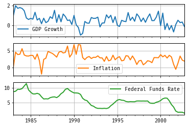
The Most Iconic Trio in Macroeconomics
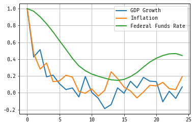
Autocorrelation
Bibliography
References
Brockwell, Peter J. and Davis, Richard A. (1987). Time Series: Theory and Methods, Springer New York.
Eugen Slutzky (1937). The Summation of Random Causes as the Source of Cyclic Processes, [Wiley, Econometric Society].
James Hamilton (1994). Time Series Analysis, Princeton University Press.
John Cochrane (2005). Time Series Analysis for Macroeconomics and Finance, Mimeo.