ECON 616: Lecture 10: Intro to Nonlinear Times Series Models

Introduction

References

Books:

• Hamilton, Chapter 21

Introduction

This week, we’ll focus on a particular kind of nonlinearity – time-varying volatiltity.

1. ARCH/GARCH models
2. Stochastic Volatility Models
3. Markov-Switching Models

ARCH/GARCH Models

ARCH

We started the course talking about autoregressive models for observables \(y_t\). Let’s allow the variance of \(y_t\) to vary over time.
The p-th order ARCH model, first used in Engle (1982)

\begin{eqnarray} \label{eq:arch} y_t &=& \mu + \epsilon_t \\ \sigma_{\textcolor{red}{t}}^2 &=& \omega + \alpha_1 \epsilon_{t-1}^2 + \ldots + \alpha_p\epsilon_{t-p}^2 \\ \epsilon_t &=& \sigma_t e_t \quad e_t \sim N(0,1). \end{eqnarray}

Key feature: variance of \(\epsilon_t\) is time varying and depends on past \(p\) shocks through their squares.
Note: \(\sigma_t\) is known at time \(t-1\)!

ARCH

This means that \[ y_{t|t-1} \sim N(\mu, \sigma_t^2) \] Since \(E_{t-1}[\epsilon_t^2] = E_{t-1}[e^2_t \sigma_t^2] = \sigma_t^2 E_{t-1}[e_t^2] = \sigma_t^2\).
What about the unconditional expectation: \(E[\sigma^2_t]\)

\begin{eqnarray*} \label{eq:uncond} E[\sigma^2_t] &=& E[\omega + \alpha_1 \epsilon_{t-1}^2 + \ldots + \alpha_p\epsilon_{t-p}^2] \\ &=& \omega + \alpha_1 E[\epsilon_{t-1}^2] + \ldots + \alpha_pE[\epsilon_{t-p}^2] \\ &=& \omega + \alpha_1 E[\sigma_{t-1}^2]E[e_{t-1}^2]+ \ldots + \alpha_pE[\sigma_{t-p}^2]E[e_{t-p}^2] \\ &=& \omega + \alpha_1 E[\sigma_{t-1}^2]+ \ldots + \alpha_pE[\sigma_{t-p}^2] \\ \end{eqnarray*}

If the unconditonal variance exists, \(\bar \sigma^2 = E[\sigma_{t-j}^2]\) for all \(j\), so \[ \bar \sigma^2 = \frac{\omega}{1 - \alpha_1 - \ldots - \alpha_p} \]

Stationarity

An ARCH(p) proces is stationary if \[ 1 - \alpha_1 - \ldots - \alpha_p > 0 \] We also require \(\alpha_j > 0\) for all \(j\). Why?
Some more analytics: Consider an ARCH(1)

\begin{eqnarray*} \label{eq:arch} y_t &=& \epsilon_t \\ \sigma_{\textcolor{red}{t}}^2 &=& \omega + \alpha_1 \epsilon_{t-1}^2 \\ \epsilon_t &=& \sigma_t e_t \quad e_t \sim N(0,1). \end{eqnarray*}

Then

\begin{eqnarray*} \sigma_{t}^2 &=& \omega + \alpha_1 \epsilon_{t-1}^2 \\ \sigma_{t}^2+\epsilon_t^2 -\sigma_t^2 &=& \omega + \alpha_1 \epsilon_{t-1}^2 +\epsilon_t^2 -\sigma_t^2 \\ \epsilon_t^2 &=& \omega + \alpha_1 \epsilon_{t-1}^2 +\epsilon_t^2 -\sigma_t^2 \\ \epsilon_t^2 &=& \omega + \alpha_1 \epsilon_{t-1}^2 +\sigma_t^2(e^2_t - 1) \\ \epsilon_t^2 &=& \omega + \alpha_1 \epsilon_{t-1}^2 +\nu_t \\ \end{eqnarray*}

ARCH(1)

\(\nu_t = \sigma_t^2(e_t^2-1)\) is the volatility surprise:

1. \(E[\nu_t] = 0\)
2. \(E[\nu_t\nu_{t-j}] = 0\)

it’s white noise!
This means that \(\epsilon_t\) follows an AR(1) like process \[ \epsilon_t^2 - \bar \sigma^2 = \sum_{j=0}^\infty \alpha_1^j \nu_{t-j} \] What does the autocorrelation function look like?

Kurtosis

Another property of ARCH models is that the kurtosis of shocks \(\epsilon_t\) is strictly greater than the kurtosis of a normal.
This might seem strange because \(\epsilon_t = \sigma_te_t\) is normal by assumption.

\begin{eqnarray*} \kappa &=& \frac{ E[\epsilon_t^4] }{E[\epsilon_t^2]^2} = \frac{ E[\sigma_t^4E_{t-1}[e_t^4]] }{E[\sigma_t^2E_{t-1}[e_t^2]]^2} = 3\frac{ E[\sigma_t^4] }{E[\sigma_t^2]^2} \end{eqnarray*}

But we know that \(V[\epsilon_t^2] = E[\epsilon_t^4] - E[\epsilon_t^2] = E[\sigma_t^4] - E[\sigma_t^2]\ge0\).

This means that \[ \frac{ E[\sigma_t^4] }{E[\sigma_t^2]^2} \ge 1 \] for \(\alpha\ne 0\) we can show this hold strictly.

GARCH

ARCH models typically require many lags to adequately model conditional variance.
Enter Generalized ARCH (GARCH), introduced by Bollerslev (1986), a parsimonious way of measuring conditional volatility,

\begin{eqnarray} \label{eq:arch} y_t &=& \mu + \epsilon_t \\ \sigma_{t}^2 &=& \omega + \sum_{j=1}^p\alpha_j \epsilon_{t-j}^2 + \textcolor{blue}{\sum_{j=1}^p\beta_j \sigma_{t-j}^2} \\ \epsilon_t &=& \sigma_t e_t \quad e_t \sim N(0,1). \end{eqnarray}

GARCH is an ARCH model with \(q\) additional lags of the conditional variance.
Call this a GARCH(p,q) model.

GARCH(1,1)

\vspace{-0.3in}

\begin{eqnarray*} \label{eq:garch} y_t &=& \epsilon_t \\ \sigma_{t}^2 &=& \omega + \alpha_1 \epsilon_{t-1}^2 + \beta_1 \sigma_{t-1}^2 \\ \epsilon_t &=& \sigma_t e_t \quad e_t \sim N(0,1). \end{eqnarray*}

We have

\begin{eqnarray*} \sigma_t^2 &=& \omega + \alpha_1 \epsilon_{t-1}^2 + \beta_1 (\omega + \alpha_1 \epsilon_{t-2}^2 + \beta_1\sigma_{t-2}^2) \\ &=& \sum_{j=0}^{\infty}\beta_1^j\omega + \sum_{j=0}^\infty \beta_1^j\alpha_1 \epsilon_{t-j-1}^2 \\ \end{eqnarray*}

Conditional variance is a constant plus a weighted average of past squared innovations.
Would need many lags to match this with an ARCH.
Parameter restrictions to ensure variances are uniformly positive? Gets very difficult for general GARCH(p,q), see Nelson and Cao (1992).

GARCH(1,1)

Time series model for \(\epsilon_t\)

\begin{eqnarray*} \sigma_{t}^2 &=& \omega + \alpha_1 \epsilon_{t-1}^2 + \beta_1 \sigma_{t-1}^2 \\ \sigma_{t}^2 + \epsilon_t^2 - \sigma_t^2 &=& \omega + \alpha_1 \epsilon_{t-1}^2 + \beta_1 \sigma_{t-1}^2 + \epsilon_t^2 - \sigma_t^2 \\ \epsilon_t^2 &=& \omega + \alpha_1 \epsilon_{t-1}^2 + \beta_1\epsilon_{t-1}^2 + \beta_1 \nu_{t-1} + \nu_t \\ \epsilon_t^2 &=& \omega + (\alpha_1+\beta_1) \epsilon_{t-1}^2 + \beta_1 \nu_{t-1} + \nu_t \end{eqnarray*}

Instead of AR(1), GARCH(1,1) is transformed into an ARMA(1,1) where \(\nu_t = \epsilon_t^2 - \sigma_t^2\) is the volatility surprise.
Unconditional Variance \[ \bar\sigma^2 = \frac{\omega}{1-\alpha_1-\beta_1} \] Autocovariances? Use formulas for autocovariances of ARMA!

More Flavors of ARCH

Exponential GARCH: [Nelson (1991)] model the natural log of variance rather the variance: \[ \ln (\sigma^2) = \omega + \sum_{j=1}\alpha_j\left(\left|\frac{\epsilon_{t-j}}{\sigma_{t-j}}\right| -\sqrt{\frac{2}{\pi}}\right) \sum_{j=1}^o\gamma_j \frac{\epsilon_{t-j}}{\sigma_{t-j}} + \sum_{j=1}^{q}\beta_j \ln(\sigma_{t-j}^2) \] No parameter restrictions!
But, more complicated form
But, possible assymetry.
Many other variants possible!

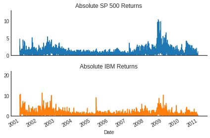
Some Data

Daily Data: 2001-2011

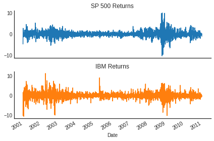
Evidence of ARCH

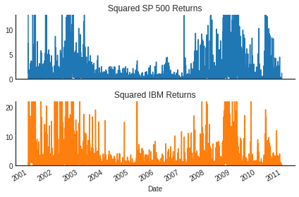
(Less Noisy) Evidence of ARCH

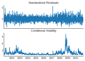
ARCH(5) for S&P 500

Constant Mean - ARCH Model Results

Dep. Variable:	SP 500 Returns	R-squared:	0.000
Mean Model:	Constant Mean	Adj. R-squared:	0.000
Vol Model:	ARCH	Log-Likelihood:	-3796.37
Distribution:	Normal	AIC:	7606.74
Method:	Maximum Likelihood	BIC:	7647.55
		No. Observations:	2515
Date:	Thu, Mar 13 2025	Df Residuals:	2514
Time:	21:09:32	Df Model:	1

Mean Model

	coef	std err	t	P>|t|	95.0% Conf. Int.
mu	-0.0379	1.862e-02	-2.035	4.189e-02	[-7.439e-02,-1.390e-03]

Volatility Model

	coef	std err	t	P>|t|	95.0% Conf. Int.
omega	0.3654	4.278e-02	8.540	1.338e-17	[ 0.282, 0.449]
alpha[1]	0.0414	2.229e-02	1.858	6.314e-02	[-2.268e-03,8.509e-02]
alpha[2]	0.1640	3.150e-02	5.205	1.940e-07	[ 0.102, 0.226]
alpha[3]	0.2090	3.437e-02	6.083	1.183e-09	[ 0.142, 0.276]
alpha[4]	0.1891	3.234e-02	5.848	4.987e-09	[ 0.126, 0.252]
alpha[5]	0.2037	3.771e-02	5.401	6.617e-08	[ 0.130, 0.278]

Covariance estimator: robust

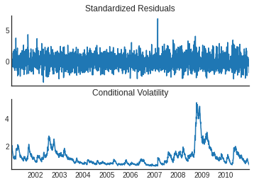
GARCH(1,1) for S&P 500

Constant Mean - GARCH Model Results

Dep. Variable:	SP 500 Returns	R-squared:	0.000
Mean Model:	Constant Mean	Adj. R-squared:	0.000
Vol Model:	GARCH	Log-Likelihood:	-3723.31
Distribution:	Normal	AIC:	7454.63
Method:	Maximum Likelihood	BIC:	7477.95
		No. Observations:	2515
Date:	Thu, Mar 13 2025	Df Residuals:	2514
Time:	21:09:33	Df Model:	1

Mean Model

	coef	std err	t	P>|t|	95.0% Conf. Int.
mu	-0.0380	1.764e-02	-2.153	3.131e-02	[-7.255e-02,-3.406e-03]

Volatility Model

	coef	std err	t	P>|t|	95.0% Conf. Int.
omega	0.0125	5.542e-03	2.253	2.429e-02	[1.622e-03,2.334e-02]
alpha[1]	0.0779	1.144e-02	6.808	9.877e-12	[5.548e-02, 0.100]
beta[1]	0.9134	1.213e-02	75.325	0.000	[ 0.890, 0.937]

Covariance estimator: robust

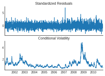
EGARCH(1,1,1) for S&P 500

ARCH(5) results

GARCH(1,1) results

EGARCH(1,1,1) results

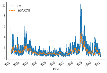
Stochastic Volatility

Stochastic Volatility

Consider the stochastic volatlity model

\begin{eqnarray} \label{eq:sv} y_t &=& \mu + \sigma_t\epsilon_t \\ \ln(\sigma_t^2) &=& \omega + \alpha_1\ln(\sigma_{t-1}^2) + \textcolor{blue}{\xi_t} \\ &~& \epsilon_t \sim N(0,1) \mbox{ and } \xi_t \sim N(0,\sigma_{\xi}^2) \end{eqnarray}

This is different from (G)ARCH: there is _volatility specific_ shock.

1. More flexible + link up better to some continuous time asset pricing models.
2. Much harder to estimate
   1. GMM: Wiggins (1987).
   2. Quasi MLE: Harvey, Ruiz, and Shephard (1994).
   3. Bayesian Approach: Jacquier, Polson, and Rossi (1994).

Connections to GARCH: see Fleming and Kirby (2003).

SV vs. GARCH

1. Some studies have found superiority of SV models of GARCH–Kim, Shephard, and Chib (1998).
2. But, of course, GARCH models are much easier to estimate.
3. Both are used.

Let’s estimate an SV model for the SP 500 returns.
I’m going to do an Bayesian analysis with \(\alpha_1 = 1\) (random walk!)

Priors: \(\mu\sim Exp(1), \sigma\sim Exp(1/0.02)\),
I’m going to use an MCMC sampler designed for this kind of model.
It takes about 20 minutes to estimate [GARCH is basically instant]

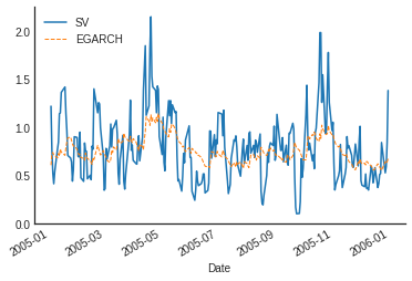
SV vs. EGARCH

SV vs. EGARCH (2005)

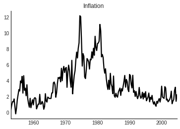
A famous SV paper…

Stock and Watson (2007): “Why Has Inflation Become Harder to Forecast?” Journal of Money, Credit, and Banking.
Has inflation become harder to forecast recently?

1. No, MSE of forecasts has gone down.
2. Yes, improvement of “structural” models relative to univariate ones have diminished.

Propose an Unobserved Components-Stochastic Volatility (UC-SV) model for inflation:

\begin{eqnarray*} \pi_t &=& \tau_t + \eta_t, \quad \eta_t \sim N(0,\sigma_{\eta,t}^2) \nonumber \\ \tau_t &=& \tau_{t-1} + \epsilon_t, \quad \epsilon_t \sim N(0,\sigma_{\epsilon,t}^2) \nonumber \\ \ln \sigma_{\eta,t}^2 &=& \ln \sigma_{\eta,t-1}^2 + \nu_{\eta,t}, \nu_t \sim N(0,\gamma^2) \nonumber \\ \ln \sigma_{\epsilon,t}^2 &=& \ln \sigma_{\epsilon,t-1}^2 + \nu_{\epsilon,t},\sim N(0,\gamma^2) \nonumber \\ \end{eqnarray*}

\(\tau_t\) = permanent (stochastic) trend inflation

\(\eta_t\) = transitory component.

Inflation

Estimation

There are no parameters to estimate, as SW set \(\gamma=0.2\).
Still have to filter the volatilities \(\{\sigma_{\eta,t}\}_{t=1}^T\) and \(\{\sigma_{\epsilon,t}\}_{t=1}^T\).
SW use a Markov-chain Monte Carlo (MCMC) technique to do this.
Compare this to a time-varying Integrated Moving Average (IMA) model:

\begin{eqnarray} \Delta\pi_t = (1-\theta_t L)e_t, \quad e_t \sim iid(0,\sigma_e^2). \end{eqnarray}

UC-SV model implies that: \[ \theta_t = \frac{1 - \sqrt{1 - 4\alpha_t^2}}{2\alpha}, \quad \alpha_t = \frac{\sigma_{\eta,t}^2}{\sigma_{\eta,t}^2+\sigma_{\epsilon,t}^2} \]

Results

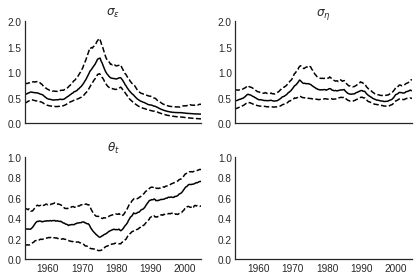
Discussion

• SD of permanent component: 1970s through 1983 = high volatility, 1950s-1960s = moderate volatility, post-83 = low volatility
  
• SD of transitory component: little change
  
• IMA estimate: moderate in early sample, falling in the 70s, increasing sharply thereafter.

Markov Switching

Markov Switching

Markov Switching – exogenous switching in parameters
Useful references:

• Hamilton, Chapter 22.
• Kim and Nelson (1999)

US GDP growth

Suppose we want to model U.S. GDP growth as a stationary AR(1): \[ y_t = \mu + \phi y_{t-1} + \epsilon_t, \quad \epsilon_{t} \sim N(0, \sigma^2). \]

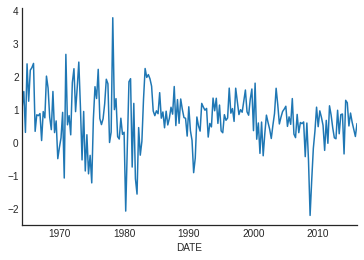
Estimation Results

We get point estimates: \((1-\hat\rho)\hat\mu = 0.5\), \(\hat\rho = 0.31\). How does it fit? Look at residuals.

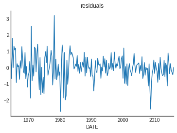
Residuals, pre and post 1984

1. The standard deviation is considerable smaller post 1984 (even with GR!)
2. While this is only suggestive, indicates there was a break in series.
3. What has broken once, can break again. How to incorporate?

Markov Switching

Let’s consider the following representation: \[ y_t = \mu(s_t) + \rho y_{t-1} + \epsilon_t, \quad \epsilon_t N(0, \sigma^2(s_t)) \] The mean and variance are now functions of an unobserved discrete random variable: \(s_t\).
Call realization of \(s_t\) the state (or regime) that discrete random variable takes.

\begin{itemize} \item $s_t = 1$, $\mu(s_t) = \mu_1, \sigma^2(s_t) = \sigma^2_1$ \item $s_t = 2$, $\mu(s_t) = \mu_2, \sigma^2(s_t) = \sigma^2_2$ \end{itemize}

We need an description for time series. A simple model is a Markov chain!

Let’s also set \(\rho=0\) for now, for simplicity.

Markov Chains, continued

We talked about Markov Chains when we talked about Markov Chain Monte Carlo. Let’s review.
Suppose \(s_t\) is an RV that takes values in \(\{1,2,\ldots,N\}\). The probabilitiy distribution for \(s_t\) depends only one the past through it’s most recent realization \(s_{t-1}\). \[ P(s_t = j | s_{t-1} = i,s_{t-2}=k,\ldots) = P(s_t = j | s_{t-1} = i) = p_{ij} \] \(p_{ij}\) is the probability of state \(j\)given state \(i\) last period.
Note that \[ \sum_{j=1}^N p_{ij} = 1, \mbox{ for } i = 1,\ldots,N. \]

Markov Chains, continued

Stack these probablity in a matrix.

\begin{equation} \label{eq:P} P = \left[ \begin{array}{cccc} p_{11} & p_{21} & \cdots & p_{N1}\\ p_{12} & p_{22} & \cdots & p_{N2} \\ \vdots & \vdots & \cdots & \vdots \\ p_{N1}& p_{N1} & \ldots & p_{NN} \end{array} \right] \end{equation}

Let \(\xi_t = [1, 0, 0, \ldots, 0]’\) when \(s_t=1\), \(\xi_t = [0, 1, 0, \ldots, 0]’\) when \(s_t=2\), and so on. This means that \[ E[\xi_{t+1}|\xi_t] = E[\xi_{t+1}|\xi_t, \xi_{t-1},\ldots] = P\xi_t. \] We represent our Markov Chain as \[ \xi_{t+1} = P\xi_t + \nu_t, \quad \nu_t = \xi_{t+1} - E[\xi_{t+1}|\xi_t] \] \(\nu_t\) is an Martingale Difference Series: mean zero and impossible to forecast using previous states.

Forecasting with Markov Chain

\begin{eqnarray*} \xi_{t+m} = \nu_{t+m} + P\nu_{t+m-1} + P^2\nu_{t+m-2} + \ldots + P^m \xi_t \end{eqnarray*}

This means that \[ E[\xi_{t+m}|\xi_t] = P^m\xi_t. \] The probability that a state from regime \(i\) will be followed \(m\) periods later by a realization of state \(j\) is given by the \(j\)th row, \(i\)th column element of \(P^m\).
Concepts:

1. reducibility: if the chain is vanishing, in the sense that once you visit a state, you will not return to some other states. Not reducible? irreducible
2. ergodicity: An irreducible MC is ergodoc, is ergodic is there exists a probability vector \(\pi\) such that \(P\pi = \pi\).

More MC

1. An ergodic Markov Chain is a covariance stationary process,
2. But, the VAR has a unit root in it!
3. Magic: the variance matrix of \(\nu_t\) is singular.

Calculating ergodic probabilty: \\[ P\pi = \pi \mbox{ and } \bf{1}'\pi = 1. \\] So

\begin{equation*} \left[ \begin{array}{c} I - P \\ \bf{1}' \end{array} \right] \pi = A\pi = e_{N+1} \end{equation*}

This means that \(\pi = (A’A)^{-1}A’e_{n+1}\).
Periodic markov chain: there is more than one \(\pi\) s.t. \(P\pi = \pi\).

Analyzing Mixtures of Normals

With \(\rho = 0\), \(y_t\) is normally distributed conditional on \(s_t\). \[ p(y_t | s_t = j; \theta) = \frac{1}{\sqrt{2\pi\sigma_j}}\exp{-\frac{(y_t - \mu_j)^2}{2\sigma^2_j}} \] We also know that \(P(A \mbox{ and } B) = P(A|B)p(B)\). So: \[ p(y_t, s_t=j;\theta) = \frac{1}{\sqrt{2\pi\sigma_j}}\exp{-\frac{(y_t - \mu_j)^2}{2\sigma^2_j}} \times p(s_t = j) \] If \(p(s_t = j;\theta) = \pi_j\), we have \[ p(y_t;\theta) = \sum_{j=1}^N\frac{1}{\sqrt{2\pi\sigma_j}}\exp{-\frac{(y_t - \mu_j)^2}{2\sigma^2_j}} \times \pi_j, \quad p(Y_{1:T};\theta) = \prod_{t=1}^T p(y_t;\theta) \] This is a mixture of normals.

Mixture of \(N(0,1)\) and \(N(2, 8)\), \(\pi_1 = 0.6\).

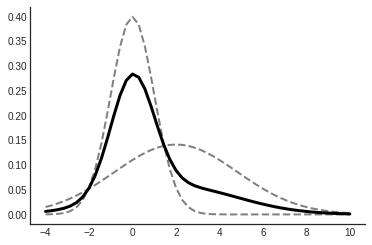
you can make some pretty crazy (any) distributions with mixture of normals.

More on Mixtures

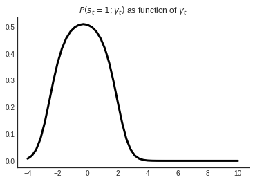
How to infer which state I’m in? Bayes Rule! \[ p(s_t = j|y_t;\theta) = \frac{p(y_t|s_t=j;\theta) p(s_t=j;\theta)}{p(y_t;\theta)} \]

How to estimate Mixtures

One can show that the MLE’s of \(\theta = [\mu, \sigma, \pi]\) are

\begin{eqnarray*} \hat \mu_j &=& \frac{\sum_{t=1}^T y_t p(s_t = j|y_t,\hat\theta)}{\sum_{t=1}^T p(s_t = j|y_t,\hat\theta)}, \quad j = 1,\ldots, N \\ \hat \sigma_j^2 &=& \frac{\sum_{t=1}^T (y_t-\hat\mu_j)^2 p(s_t = j|y_t,\hat\theta)}{\sum_{t=1}^T p(s_t = j|y_t,\hat\theta)}, \quad j = 1,\ldots, N \\ \hat \pi &=& \frac{1}{T} \sum_{t=1}^T p(s_t = j|y_t,\hat\theta) \end{eqnarray*}

Recall, we get \(p(s_t=j|y_t,\theta)\) from applying Bayes rule.
This forms a system of nonlinear equations, which in principal can be solved.
Another way…

The EM Algorithm

A simple iterative procedure:

1. Guess arbitrary \(\hat\theta^0\),
2. Plugin in to RHS of above equations, get \(\hat\theta^1\)
3. if \(|\hat\theta^1 - \hat\theta^0| < \epsilon\), you’ve found a maximum
4. otherwise continuing iterating

This is called the _EM Algorithm._

1. Each iteration increases the value of the likelihood function
2. Usually works very fast
3. Not guaranteed to find a global max, but generally robust.

Issues in optimization

1. if \(\hat\mu_j = y_t\) for some j and \(y_t\), we’re in trouble, because the max will send \(\sigma_j \rightarrow 0\).

2. This makes the log-likelihood go to infinity

3. More generally: there is a labeling issue: \((\mu_1, \sigma_1^2)\) could easily be called \((\mu_2, \sigma_2^2)\) and vice versa.

4. This calls for augmenting the problem with more information.

   1. Coherent way: Bayesian Approach, see Kim and Nelson (1999).
   2. Ad hoc way: augment the likliehood with a penalty function to enforce priors views and make pathologies less likely. See Hamilton (1994).

Markov Switching

Markov Switching models are more complicated versions of the mixture model.
Instead of just \(\pi = [\pi_1, \ldots, \pi_N]\) we need to estimate \(P\)

\begin{equation} P = \left[ \begin{array}{cccc} p_{11} & p_{21} & \cdots & p_{N1}\\ p_{12} & p_{22} & \cdots & p_{N2} \\ \vdots & \vdots & \cdots & \vdots \\ p_{N1}& p_{N1} & \ldots & p_{NN} \end{array} \right] \end{equation}

Key item is again: distribution of states conditional on data.
Now we need to consider entire history of data, because of Markovian structure. \[ \hat\xi_{t|t} = [p(s_t = 1|Y_{1:t};\theta), \ldots, p(s_t = N|Y_{1:t-1};\theta)]' \] We can also think about the forecast of this probability distribution \[ \hat\xi_{t|t-1}. \]

Deriving the likelihood

The joint distribution of \(y_t\) and \(s_t\) given \(Y_{1:t-1}\) is given by \[ p(y_t,s_t=j|Y_{1:t-1};\theta) = p(y_t|s_{t}=j,Y_{1:t-1};\theta)p(s_{t}=j|Y_{1:t-1};\theta) \] Let \(\eta_t = [p(y_t|s_{t}=1,Y_{1:t-1};\theta), \ldots, p(y_t|s_{t}=N,Y_{1:t-1};\theta)]’\).
Recall \(\hat\xi_{t|t-1} = [p(s_t = 1|Y_{1:t-1};\theta), \ldots, p(s_t = N|Y_{1:t-1};\theta)]’\)
Then \(p(y_t,s_t=j|Y_{1:t-1};\theta) = \hat\xi_{t|t-1}\odot \hat\eta_{t}\).
\[ p(y_t|Y_{1:t-1};\theta) = \sum_{j=1}^N p(y_t,s_t=j|Y_{1:t-1};\theta) = {\bf 1}’ (\hat\xi_{t|t-1}\odot \eta_t) \] The log likelihood is \[ \sum_{j=1}^T log p(y_t|Y_{1:t-1};\theta) = \sum_{t=1}^T log\left({\bf 1}’ (\hat\xi_{t|t-1}\odot \eta_t)\right) \] Now to get a recursion for \(\hat\xi_{t|t-1}\)

Recursion for \(\hat\xi_{t|t-1}\)

Use Bayes rule \[ p(s_t=j|Y_{1:T};\theta) = \frac{p(y_t|s_{t}=j;\theta)p(s_t=j|Y_{1:t-1};\theta)} {p(y_t|Y_{1:t-1};\theta)} \] Which is just \[ p(s_t=j|Y_{1:T};\theta) = \hat \xi_{t|t} = \frac{(\hat\xi_{t|t-1}\odot \eta_t)}{{\bf 1}’ (\hat\xi_{t|t-1}\odot \eta_t)} \] To get forecast: \[ E_t[\xi_{t+1}|Y_{1:T}] = PE_t[\xi_t|Y_{1:T}] + E_t[\nu_t|Y_{1:T}] = P\hat\xi_{t|t} \] And we’re done!

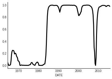
Smoothed Probabilities

Kim Algorithm:
Do this stuff ``backwards’’: \[ \hat\xi_{t|T} = \hat\xi_{t|t} \odot [P’ [\hat \xi_{t+1} / \hat \xi_{t+1|t}] ] \] Estimation

1. Hamilton: If initial probablities are unrelated \[ \hat p_{ij} = \frac{\sum_{t=2}^T p(s_t = j, s_t = i| Y_{1:T};\theta)}{\sum_{t=2}^Tp(s_{t-1} = i;Y_{1:T}\theta)} \]
2. Otherwise, a bit more complicated
3. either way use EM algorithm.

Back to Example

Markov Switching Model Results

Dep. Variable:	GDPC1	No. Observations:	207
Model:	MarkovAutoregression	Log Likelihood	-220.722
Date:	Thu, 13 Mar 2025	AIC	455.444
Time:	21:14:01	BIC	478.773
Sample:	04-01-1964	HQIC	464.878
	- 01-01-2016
Covariance Type:	approx

Regime 0 parameters

	coef	std err	z	P>|z|	[0.025	0.975]
const	0.7393	0.066	11.280	0.000	0.611	0.868
sigma2	0.2301	0.035	6.557	0.000	0.161	0.299

Regime 1 parameters

	coef	std err	z	P>|z|	[0.025	0.975]
const	0.7114	0.168	4.239	0.000	0.382	1.040
sigma2	1.1565	0.197	5.862	0.000	0.770	1.543

Non-switching parameters

	coef	std err	z	P>|z|	[0.025	0.975]
ar.L1	0.2834	0.074	3.847	0.000	0.139	0.428

Regime transition parameters

	coef	std err	z	P>|z|	[0.025	0.975]
p[0->0]	0.9792	0.018	53.932	0.000	0.944	1.015
p[1->0]	0.0289	0.027	1.071	0.284	-0.024	0.082

Warnings:
[1] Covariance matrix calculated using numerical (complex-step) differentiation.

Smoothed Probabilities

Bibliography

References

References