ECON 616: Lecture Three: The Spectrum
Intro
Background
Overview: Chapters 6 from Hamilton (1994).
Technical Details: Chapter 4 from Brockwell and Davis (1987).
Other stuff: You might want to look at a digital signals processing textbook, for example: here.
Cycles as Frequencies
Starting In the 19th Century, economists and others recognized cyclical patterns in economic activity.
Schmupeter distinguished between cycles at different frequencies
- Kondratieff Cycles – Longwave cycles lasting 50 years (caused by fundamental innovations.)
- Juglar Cycles – medium cycle (8 years) associated with changes in credit condition.
- Kitchin Cycles – short run cycles (40 months) associated with information diffusion.
=> model economic activity as a linear combination of periodic function with different frequencies.
A model of frequencies
Consider the following model for quarterly observations \[ X_t = 2 \sum_{j=1}^m a_j cos( \omega_j t + \theta_j) \] where \(\theta_j\) is \(\sim iidU[-\pi,\pi]\) and \(-\pi \le \omega_j < \omega_{j+1} \le \pi\). The random variables \(\theta_j\) are determined in the infinite past and simply cause a phase shift. According to Schumpeter’s hypothesis \(m\) should be equal to three. The frequencies \(\omega_j\) can be determined as follows.
| Cycle | Duration | Frequency |
|---|---|---|
| Kondratieff | 200 quarters | \(\omega_1 = (2 \pi)/200 = 0.03\) |
| Juglar | 32 quarters | \(\omega_2 = (2\pi)/32 = 0.20\) |
| Kitchin | 13.3 quarters | \(\omega_3 = (2 \pi)/13.3 = 0.47\) |
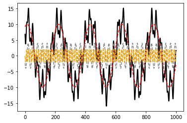
A Time Series of this process
\(a = [5,2,1], \quad \omega = [0.03,0.20,047]\).
The Spectrum
The coefficients \(a_1\) to \(a_3\) are the amplitudes of the different cycles
If \(a_1\) and \(a_2\) are small then most of the variation in \(X_t\) is due to the Kitchin cycles.
The plot of \(a_j^2\) versus \(\omega\) is called the spectrum of \(X_t\).
Some math
\begin{eqnarray} \cos(x+y) & = & \cos x \cos y - \sin x \sin y \\ \sin x \sin y & = & \frac{1}{2} [ \cos(x-y) - \cos(x+y)] \\ \cos x \cos y & = & \frac{1}{2} [ \cos(x-y) + \cos(x+y)] \\ 2 \sin^2 x & = & 1 - \cos (2x) \\ \sin x \cos x & = & \frac{1}{2} \sin (2x) \end{eqnarray}
Moreover, \(\sin^2 x + \cos^2 x = 1\).
We consider real-valued stochastic processes \(X_t\), complex numbers will help us summarize sine and cosine expressions using exponential functions.
More Math
Let \(i = \sqrt{-1}\).
Euler’s formula: \[ e^{i \varphi} = \cos \varphi + i \sin \varphi \] The formula becomes less mysterious if you rewrite \(e^{i\varphi}\), \(\sin \varphi\), and \(\cos \varphi\) as power series.
The Plan
Rewrite Schumpeter Model
Define spectral distribution / density function
Examine relationship between autocovariances \(\{\gamma_h\}_{h=-\infty}^\infty\) and the spectrum.
Discuss very general spectral representation for a stationary stochastic process \(X_t\).
Schumpeter Model
\[ X_t = 2 \sum_{j=1}^m a_j \cos \theta_j \cos(\omega_j t) - a_j \sin \theta_j \sin(\omega_j t) \]
where \(a_j \cos \theta_j\) and \(a_j \sin \theta_j\) can be regarded as random coefficients.
Eulers formula implies
\[ X_t = \sum_{j=-m}^m A(\omega_j) e^{i \omega_j t} \]
where \(\omega_{-j} = -\omega_j\). Let \(a_{-j} = a_j\) and
This means that
\[ A(\omega_j) = \left\{ \begin{array}{ll} a_j( \cos \theta_{|j|} + i \sin \theta_{|j|} ) & \mbox{if} \; j > 0 \\ a_j( \cos \theta_{|j|} - i \sin \theta_{|j|} ) & \mbox{if} \; j < 0 \\ \end{array} \right. \]
We can verify that:
\[ A(\omega_j) e^{i \omega_j t} + A(\omega_{-j}) e^{- i \omega_j t} = 2 \left[ a_j \cos \theta_j \cos(\omega_j t) - a_j \sin \theta_j \sin(\omega_j t) \right] \]
Moments of Linear Cyclical Models
\begin{eqnarray} \mathbb E[\cos \theta_j] &=& \frac{1}{2\pi} \int_{-\pi}^\pi \cos \theta_j d\theta_j = 0 \\ \mathbb E[\sin \theta_j] &=& \frac{1}{2\pi} \int_{-\pi}^\pi \sin \theta_j d\theta_j = 0 \end{eqnarray}
Result: The expectation of \(X_t\) in the linear cyclical model is equal to zero. \(\Box\)
Autocovariances
To obtain the autocovariances \(\gamma_h = \mathbb E[X_tX_{t-h}]\) we have to calculate the moments \(\mathbb E[ A(\omega_j) A(\omega_k)]\).
Let \(j \not=k\), \(j \not=-k\). Suppose that \(j,k > 0\).
\begin{eqnarray} \mathbb E[A(\omega_j) A(\omega_k)] & = & a_ja_k\mathbb E[ (\cos \theta_j + i \sin \theta_j)(\cos \theta_k + i \sin \theta_k)] \nonumber \\ & = & a_ja_k\mathbb E[ \cos \theta_j \cos \theta_k + i \cos \theta_j \sin \theta_k i\cos \theta_k \sin \theta_j - \sin \theta_j \sin \theta_k ] \nonumber \\ & = & 0 \end{eqnarray}
Since \(\theta_j\) and \(\theta_k\) are independent. Similar arguments can be made if \(j\) and \(k\) have different signs.
Covariance
Let \(j=k\). Suppose that \(j,k > 0\).
\begin{eqnarray} \mathbb E[A(\omega_j) A(\omega_k)] & = & a_j^2 \mathbb E[ (\cos \theta_j + i \sin \theta_j)^2] \nonumber \\ & = & a_j^2 \mathbb E[ (\cos^2 \theta_j - \sin^2 \theta_j + i 2 \cos \theta_j \sin \theta_j ] \nonumber \\ & = & a_j^2 \mathbb E[ 1 - 2\sin^2 \theta_j + i2 \cos \theta_j \sin \theta_j ] \nonumber \\ & = & a_j^2 \mathbb E[ \cos (2\theta_j) + i \sin (2 \theta_j) ] \nonumber \\ & = & 0 \end{eqnarray}
In the last step we use the fact that sine and cosine integrate to zero over two cycles. A similar argument can be made for the case \(j,k < 0\)
Let \(j=-k\). Now \(A(\omega_j)\) and \(A(\omega_{k})\) are complex conjugates. \[ \mathbb E[A(\omega_j) A(\omega_{-j})] = a_j^2 \mathbb E[ \cos^2 \theta_j + \sin^2 \theta_j] = a_j^2 \]
The upshot
Result: The autocovariances of the process \(X_t\) generated by the linear cyclical model are given by
\begin{eqnarray} \gamma_h & = & \mathbb E[X_t X_{t-h}] \nonumber \\ & = & \sum_{j=-m}^m \sum_{k=-m}^m \mathbb E[ A(\omega_j)A(\omega_k)] e^{i\omega_j t} e^{i \omega_k(t-h)} \nonumber \\ & = & \sum_{j=-m}^m \mathbb E[A(\omega_j) \overline{A(\omega_j)}] e^{i \omega_j h} = \sum_{j=-m}^m a_j^2 e^{i \omega_j h} \end{eqnarray}
Since \(X_t\) is a real valued process the autocovariances can also be written as \[ \gamma_h = 2 \sum_{j=1}^m a_j^2 \cos(\omega_j h) \quad \Box \]
The Spectral Distribution
The spectral distribution function for the process \(X_t\), defined on the interval \(\omega \in (-\pi,\pi)\), is \[ S(\omega) = \sum_{j=-m}^m \mathbb E[A(\omega_j) \overline{A(\omega_j)} ] \{\omega_j \le \omega\} \] where \(\{ \omega_j \le \omega\}\) denotes the indicator function that is one if \(\omega_j \le \omega\). \(\Box\)
Remarks
The spectral distribution is non-negative and continuous from the right.
If the spectral distribution function is evaluated at \(\omega=\pi\) we obtain
\begin{eqnarray} S(\pi) = \sum_{j=-m}^m \mathbb E[A(\omega_j) \overline{A(\omega_j)} ] = \sum_{j=-m}^m a_j^2 = \mathbb E[X_t^2] \end{eqnarray}
The spectral distribution function is symmetric in the sense that for \(\omega >0\)
\begin{eqnarray} S(-\omega) = S(\pi) - \lim_{n \rightarrow \infty} S( (\omega - 1/n)) \end{eqnarray}
Autocovariances, again
The representation of the autocovariances can be expressed as a Riemann-Stieltjes integral. Define a sequence of grids \[ [\omega]^{(n)} =\{ \omega_k^{(n)} = 2 \pi k/n - \pi \} \] and \(\Delta_n \omega = \omega_{k+1}^{(n)} - \omega_k^{(n)} = 2\pi /n\). Moreover, let \[ \Delta_n S(\omega) = S(\omega) - S(\omega - \Delta_n \omega) \] Roughly, \[ \sum_{k=0}^n e^{i\omega_k^{(n)}h} \Delta_n S(\omega_k^{(n)}) \longrightarrow \sum_{j=-m}^m a_j^2 e^{i\omega_jh} \] as \(n \rightarrow \infty\).
The Upshot
Thus, we can express the autocovariance \(\gamma_h\) as the following integral \[ \gamma_h = \int_{(-\pi,\pi]} e^{i\omega h} dS(\omega) \]
By using a similar argument, we can also obtain a integral representation for the stochastic process \(X_t\). Define the stochastic process \[ Z(\omega) = \sum_{j=-m}^m A(\omega_j) \{\omega_j \le \omega \} \] with orthogonal increments \(\Delta_n Z(\omega) = Z(\omega) - Z(\omega - \Delta_n \omega)\). Note that the increments are now random variables.
Very roughly, \[ \sum_{k=0}^n e^{i\omega_k^{(n)} t} \Delta_n Z(\omega_k^{(n)}) \longrightarrow \sum_{j=-m}^m A(\omega_j) e^{i\omega_j t} \] almost surely as \(n \rightarrow \infty\). Thus, we can express the stochastic process \(X_t\), generated from the linear cyclical model, as the stochastic integral \[ X_t = \int_{(-\pi,\pi]} e^{i\omega t} dZ(\omega) \]
Spectral Representation for Stationary Processes
Every zero-mean stationary process has a representation of the form \[ X_t = \int_{(-\pi,\pi]} e^{i\omega h} dZ(\omega) \] where \(Z(\omega)\) is a orthogonal increment process. Correspondingly, its autocovariance function \(\gamma_h\) can be expressed as \[ \gamma_h = \int_{(-\pi,\pi]} e^{i\omega h} dS(\omega) \] where \(S(\omega)\) is a non-decreasing right continuous function with \(S(\pi) = \mathbb E[X_t^2] = \gamma_0\).
Spectral Density Function
Suppose the spectral distribution function is differentiable with respect to \(\omega\) on the interval \((-\pi,\pi]\). The spectral density function is defined as \[ s(\omega) = dS(\omega)/d\omega \] If a process has a spectral density function \(s(\omega)\) then the covariances can be expressed as \[ \gamma_h = \int_{(-\pi,\pi]} e^{ih\omega} s(\omega)d\omega \] The spectral density uniquely determines the entire sequence of autocovariances. Moreover, the converse is also true.
Consider the sum
\begin{eqnarray} s_n(\omega)^* & = & \frac{1}{2\pi}\sum_{h = -n}^n \gamma_h e^{- i \omega h} \nonumber \\ & = & \frac{1}{2\pi} \sum_{h = -n}^n \left[ \int_{(-\pi,\pi]} e^{i\tau h} s(\tau) d\tau \right] e^{-i\omega h} \end{eqnarray}
The sum \(s_n^*(\omega)\) is a Fourier series. If the spectral density \(s(\omega)\) is piecewise smooth then \[ s_n^*(\omega) \longrightarrow s(\omega) \] Thus, the spectral density can be obtained by evaluating the autocovariance generating function of \(X_t\) at \(z=e^{-i\omega}\). \[ s (\omega) = \frac{1}{2 \pi} \gamma(e^{-i\omega} ) = \frac{1}{2 \pi} \sum_{h=-\infty}^\infty \gamma_h e^{-i\omega h} \] where \[ \gamma(z) = \sum_{j=-\infty}^\infty \gamma_j z^j \]
Filter
Suppose \(s_{X}(\omega)\) is the spectral density function of a process \(X_t\). Filters are used to dampen or amplify the spectral density at certain frequencies. The spectrum of the filtered series \(Y_t\) is given by
\[ s_{Y}(\omega) = f(\omega) s_{X}(\omega). \]
where \(f(\omega)\) is the filter function.
Frequency domain trend/cycle analogue
\(X_t =\) low frequency component + high frequency component
Example: For Schumpeter, Kitchin cycle was shortest with \(\omega = 0.47\). To remove the effects of other cycles from data, we could use the filter \[ f(\omega) = \left\{ \begin{array}{ll} 0 & \mbox{if} \; \omega < 0.4 \\ 1 & \mbox{otherwise} \end{array} \right. \]
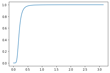
Hodrick Prescott filter
A popular filter in the real business cycle literature in macro-economics is the so-called Hodrick Prescott filter.
\[ f^{HP}(\omega) = \left[\frac{16\sin^4(\omega/2)}{1/1600 + 16\sin^4(\omega/2)}\right]^2. \]
This filter basically kills long cycles and attenuates medium term ones.
(See Soderlind, 1994.)
HP Filter
f(2pi/64) = 0.016697846612617945 f(2pi/32) = 0.4937014515264561 f(2pi/16) = 0.9481735523836959
More on Filters
Subsquently we will consider filters that are linear in the time domain, namely, filters of the form, \[ Y_t = \sum_{h=1}^J c_h X_{t-h} = C(L) X_t \] where \(C(z)\) is the polynomial function \(\sum_{h=1}^J c_h z^h\). Recall that \[ X_t = \sum_{j=-m}^m A(\omega_j) e^{i\omega_j t} \]
This means that
Hence, \[ X_{t-h} = \sum_{j=-m}^m A(\omega_j) e^{i\omega_j t} e^{-i\omega_j h} \]
\begin{eqnarray} Y_t = C(L)X_t & = & \sum_{h=1}^J c_h X_{t-h} \nonumber \\ & = & \sum_{j=-m}^m \left[ A(\omega_j) e^{i\omega_j t} \sum_{h=1}^J c_h e^{-i\omega_j h} \right] \nonumber \\ & = & \sum_{j=-m}^m A(\omega_j) C(e^{-i\omega_j}) e^{i\omega_j t} \nonumber \\ & = & \sum_{j=-m}^m \tilde{A}(\omega_j) e^{i\omega_j t} \end{eqnarray}
Autocovariance
The autocovariances of \(Y_t\) can therefore be expressed as \[ \mathbb E[Y_t Y_{t-h}] = \sum_{j=-m}^m a_j^2 C(e^{-i\omega_j}) C(e^{i\omega_j}) e^{i \omega_j h} \] Thus, we can define the spectral distribution function of \(Y_t\) as \[ S_Y (\omega) = \sum_{j=-m}^m a_j^2 C(e^{-i\omega_j}) C(e^{i\omega_j}) \] with increments \[ \Delta S_Y (\omega_j) = \Delta S_X C(e^{-i\omega_j}) C(e^{i\omega_j}) \]
Generalization
Result: Suppose that \(X_t\) has a spectral density function \(s_X(\omega)\) and \(Y_t = C(L)X_t\), then the spectral density of the filtered process \(Y_t\) is given by
\[ s_Y (\omega) = | C(e^{-i\omega}) |^2 s_X(\omega) \]
The function \(C(e^{-i\omega})\) is called transfer function of the filter, and the filter function \(f(\omega) = | C(e^{-i\omega}) |^2\) is often called power transfer function. \(\Box\)
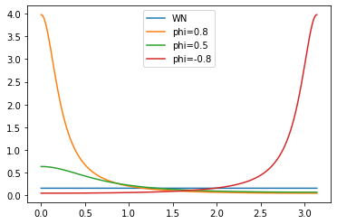
Examples of Spectrum
White Noise \[ s(\omega) = \frac{1}{2\pi}\sum_{h=-\infty}^\infty \gamma_h e^{-i\omega h} = \frac{\gamma_0}{2\pi} \] An AR(1): \(Y_t = \phi Y_{t-1} + X_t\)
Interpret as a linear filter with \(MA(\infty)\) rep: \(Y_t = \sum_{h=0}^\infty \phi^h X_{t-h}\). Thus:
\begin{eqnarray} | C(e^{-i\omega}) |^2 & = & \left| [ 1 - \phi e^{-i\omega}]^{-1} \right|^2 \nonumber \\ & = & \left[ | 1 - \phi \cos \omega + i \phi \sin \omega |^2 \right]^{-1} \nonumber \\ & = & \left[ (1 - \phi \cos \omega)^2 + \phi^2 \sin^2 \omega \right]^{-1} \nonumber \\ & = & \left[ 1 - 2 \phi \cos \omega + \phi^2( \cos \omega^2 + \sin^2 \omega ) \right]^{-1}. \end{eqnarray}
which means \(s_Y(\omega) = \frac{\sigma^2 / 2\pi }{1 + \phi^2 - 2\phi \cos \omega}\). Note \(s_Y(0) \longrightarrow \infty \; \mbox{as} \; \phi \longrightarrow 1\)
More Examples
Stationary ARMA process*: \(\phi(L)Y_t = \theta(L)X_t\) with \(X_t \sim WN\). The spectral density is given by \[ s_Y(\omega) = \left| \frac{ \theta(e^{-i\omega}) }{ \phi(e^{-i\omega}) } \right|^2 \sigma^2 \] Sums of processes. Suppose that \(W_t = Y_t + X_t\). The spectrum of the process \(W_t\) is simply the sum \[ s_W(\omega) = s_Y(\omega) + s_X(\omega) \]
Visual
<matplotlib.legend.Legend at 0x7fb821cf9f10>
Estimation
Parametric – Pick an ARMA process, estimate in time domain, use filtering results to get spectrum.
Nonparametric – Estimate autocovariances \(\{\hat \gamma_h\}\), directly write down spectral density. Let’s look at this.
Let \(\bar{y} = \frac{1}{T} \sum y_t\) and define the sample covariances \[ \hat{\gamma}_h = \frac{1}{T} \sum_{t=h+1}^T (y_t - \bar{y})(y_{t-h} - \bar{y}) \] An intuitively plausible estimate of the spectrum is the sample periodogram
\begin{eqnarray} I_T(\omega) & = & \frac{1}{2\pi} \sum_{j=-T+1}^{T-1} \hat{\gamma}_h e^{-i \omega h} \nonumber \\ & = & \frac{1}{2\pi} \left( \hat{\gamma}_0 + 2 \sum_{h=1}^{T-1} \hat{\gamma}_{h} \cos(\omega h) \right) \end{eqnarray}
Result: The sample periodogram is an asymptotically unbiased estimator of the population spectrum, that is,
\begin{equation} \mathbb E[ I_T(\omega)] \stackrel{p}{\longrightarrow} s(\omega) \end{equation}
However, it is inconsistent since the variance \(var[I_T(\omega)]\) does not converge to zero as the sample size tends to infinity. \(\Box\)
Smoothed Periodogram
Smoothing: get non-parametric estimators.
To obtain a spectral density estimate at the frequency \(\omega = \omega_*\) we will compute the sample periodogram \(I_T(\omega)\) for some \(\omega_j\)’s in the neighborhood of \(\omega_*\) and simply average them. Define the following band around \(\omega_*\):
\begin{equation} B (\omega_*|\lambda) = \left\{ \omega: \omega_* - \frac{\lambda}{2} < \omega \le \omega_* + \frac{\lambda}{2} \right\} \end{equation}
The bandwidth is \(\lambda\), where \(\lambda\) is a parameter. Moreover, define the ``fundamental frequencies’’ (see Hamilton 1994, Chapter 6.2, for a discussion why these frequencies are ``fundamental’')
\begin{equation} \omega_j = j \frac{2 \pi}{T} \quad j = 1,\ldots, (T-1)/2 \end{equation}
iThe number of fundamental frequencies in the band \(B(\omega_*)\) is
\begin{equation} m = \lfloor \lambda T(2\pi)^{-1} \rfloor \end{equation}
Smoothed Periodogram
The smoothed periodogram estimator of \(s(\omega_*)\) is defined as the average
\begin{equation} \hat{s}(\omega) = \sum_{j=1}^{(T-1)/2} \frac{1}{m} \{ \omega_j \in B(\omega_*|\lambda) \} I_T(\omega_j) \end{equation}
where \(\{ \omega_j \in B(\omega_*|\lambda) \}\) is the indicator function that is equal to one if \(\omega_j \in B(\omega_*|\lambda)\) and zero otherwise.
Result: The smoothed periodogram estimator \(\hat{s}(\omega_*)\) of \(s(\omega_*)\) is consistent, provided that the bandwidth shrinks to zero, that is, \(\lambda \rightarrow 0\) as \(T \rightarrow \infty\) and the number of \(\omega_j\)’s in the band \(B(\omega_*|\lambda)\) tends to infinity, that is $ m = λ T/(2π) → ∞$. \(\Box\)
Remarks
- get smoothed estimates => need to get \(\lambda\). Ultimately subective.
- Most non-parameterics approaches are based on “Kernel estimates”
The expression \(\{ \omega_j \in B(\omega_*) \}\) can be rewritten as follows
\begin{eqnarray} \{ \omega_j \in B(\omega_*) \} & = & \left\{ \omega_* - \frac{\lambda}{2} < \omega_j \le \omega_* + \frac{\lambda}{2} \right\} \nonumber \\ & = & \left\{ - \frac{1}{2} < \frac{\omega_j - \omega_*}{\lambda } \le \frac{1}{2} \right\} \end{eqnarray}
Define
\begin{eqnarray} K \left( \frac{\omega_j - \omega_*}{\lambda} \right) = \left\{ - \frac{1}{2} < \frac{\omega_j - \omega_*}{\lambda} \le \frac{1}{2} \right\} \end{eqnarray}
It can be easily verified that
\begin{eqnarray} \int K \left( \frac{\omega_j - \omega_*}{\lambda} \right) d\omega_* = 1 \end{eqnarray}
The function \(K \left( \frac{\omega_j - \omega_*}{\lambda} \right)\) is an example of a Kernel function. In general, a Kernel has the property \(\int K(x) dx = 1\). Since \(m \approx \lambda (T-1)/2\), the spectral estimator can be rewritten as
\begin{eqnarray} \hat{s}(\omega) = \frac{\pi }{ \lambda (T-1)/2} \sum_{j=1}^{(T-1)/2} K \left( \frac{\omega_j - \omega_*}{\lambda} \right) I_T(\omega_j) \end{eqnarray}
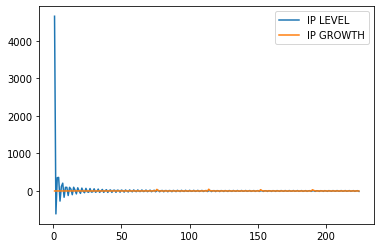
Application: IP
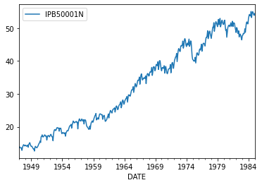
<matplotlib.legend.Legend at 0x7fb80fc883d0>
Application: Autocorrelation Consistent Standard Errors
Consider the model
\begin{equation} y_t = \beta x_t + u_t, \quad u_t = \psi(L)\epsilon_t, \quad \epsilon_t \sim iid(0,\sigma^2) \end{equation}
The OLS estimator is given by
\begin{equation} \hat{\beta} - \beta = \frac{ \sum x_t u_t}{\sum x_t^2} \end{equation}
The conventional standard error estimates for \(\hat{\beta}\) are inconsistent if the \(u_t\)’s are serially correlated. However, we can construct a consistent estimate based on non-parametric spectral density estimation. Define \(z_t = x_t u_t\). We want to obtain an estimate of
\begin{equation} \mbox{plim} \; \Lambda_T = \mbox{plim} \; \frac{1}{T} \sum_{t=1}^T \sum_{h=1}^T E[z_t z_h] \end{equation}
It can be verified that
\begin{equation} \sum_{h=-\infty}^\infty \gamma_{zz,h} - \frac{1}{T} \sum_{t=1}^T \sum_{h=1}^T E[z_t z_h] \stackrel{p}{\longrightarrow} 0 \end{equation}
Since
\begin{equation} s(\omega) = \frac{1}{2\pi} \sum_{h=-\infty}^\infty \gamma_{zz,h} e^{-i \omega h} \end{equation}
it follows that a consistent estimator of plim \(\Lambda_T\) is
\begin{equation} \hat{\Lambda}_T = 2 \pi \hat{s}(0) \end{equation}
where \(\hat{s}(0)\) is a non-parametric spectral estimate at frequency zero.
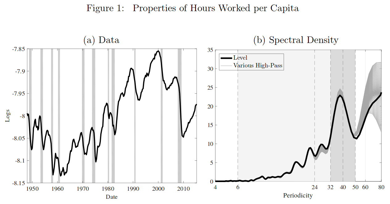
Application: Beaudry, Galizia, and Portier (2020)
Paul Beaudry, Dana Galiza, and Franck Portier (2016): “Putting the Cycle Back into Business Cycle Analysis,” NBER Working Paper.
- Re-examines the spectral properties of several cyclically sensitive variables such as hours worked, unemployment and capacity utilization.
- Document the presence of an important peak in the spectral density at a periodicity of approximately 36-40 quarters.
- This is cyclical phenomena at the “long end” of the business cycle.
- Suggests a model (“limit cycles”) to account for this finding.
The Paper in 1 Picture