ECON 616: Lecture Two: Deterministic Trends, Nonstationary Processes
Intro
Background
- Overview: Chapters 15-16 from Hamilton (1994).
- Technical Details: Davidson and MacKinnon (2003)
Trends vs Cycles
A commond decomposition of macroeconomic time series is into trend and cycle.
If \(Y^T\) corresponds to real per capita GDP \(gdp_t\) of the United States. According to this components approach to time series, \(y_t\) is expressed as \[ y_t = \ln gdp_t = trend_t + fluctuations_t \] we will examine regression techniques that decompose \(y_t\) in a trend and a cyclical component.
An identification problem
what features of the time series do we regard as trend and what do
we regard as fluctuations around the trend?
Let’s guess a linear deterministic time trend:
\[ y_t = \beta_1 + \beta_2 t + u_t \]
A decomposition of \(y_t\) into trend and fluctuations can be obtained by estimating \(\beta_1\) and \(\beta_2\):
\begin{eqnarray} y_t &=& \widehat{trend}_t + \widehat{fluctuations}_t \nonumber \\ &=& (\hat{\beta}_1 + \hat{\beta}_2 t) + ( y_t - \hat{\beta}_1 - \hat{\beta}_2t). \end{eqnarray}
When \(y_t\) is logged, the coefficient \(\beta_2\) has the interpretation of an average growth rate.
A Trend Cycle Decomposition of Log US GNP
[0;31m---------------------------------------------------------------------------[0m
[0;31mNameError[0m Traceback (most recent call last)
[0;32m<ipython-input-1-bf73901e5db8>[0m in [0;36m<module>[0;34m[0m
[1;32m 20[0m [0;31m# Assign the inferred column names[0m[0;34m[0m[0;34m[0m[0;34m[0m[0m
[1;32m 21[0m [0mdata[0m[0;34m.[0m[0mcolumns[0m [0;34m=[0m [0mcolumn_names[0m[0;34m[0m[0;34m[0m[0m
[0;32m---> 22[0;31m [0mdata[0m[0;34m[[0m[0;34m'Year'[0m[0;34m][0m [0;34m=[0m [0mp[0m[0;34m.[0m[0mto_datetime[0m[0;34m([0m[0mdata[0m[0;34m[[0m[0;34m'Year'[0m[0;34m][0m[0;34m,[0m [0mformat[0m[0;34m=[0m[0;34m'%Y'[0m[0;34m)[0m[0;34m[0m[0;34m[0m[0m
[0m[1;32m 23[0m [0mdata[0m [0;34m=[0m [0mdata[0m[0;34m.[0m[0mreplace[0m[0;34m([0m[0;36m0[0m[0;34m,[0m [0mnp[0m[0;34m.[0m[0mnan[0m[0;34m)[0m[0;34m.[0m[0mset_index[0m[0;34m([0m[0;34m'Year'[0m[0;34m)[0m[0;34m.[0m[0mto_period[0m[0;34m([0m[0;34m'A'[0m[0;34m)[0m[0;34m[0m[0;34m[0m[0m
[1;32m 24[0m [0;32mfor[0m [0mc[0m [0;32min[0m [0mdata[0m[0;34m.[0m[0mcolumns[0m[0;34m:[0m[0;34m[0m[0;34m[0m[0m
[0;31mNameError[0m: name 'p' is not defined
Deterministic Trend Model
Consider the deterministic trend model
\[
y_t = \beta_1 + \beta_2 t + u_t
\]
with \(\mathbb E[u_t]=0\) and \(var[u_t] = \sigma^2\).
There are several difficulties associated with the large sample analysis
of the OLS estimators \(\hat{\beta}_{1,T}\) and \(\hat{\beta}_{2,T}\). Taking \(x_t = [1, t]’\),
The matrix \(\frac{1}{T} \sum x_t x_t’\) does not converge to a non-singular matrix \(Q\).
In a time series model, the disturbances \(u_t\) are in general dependent. This will change the limiting distribution of quantities such as \(\sqrt{T} \frac{1}{T} \sum x_t u_t\).
If the \(u_t\)’s are serially correlated, then the OLS estimator will in general be inefficient.
Asymptotic Stuff
Rates of Convergence for OLS Estimator
Roughly speaking, convergence rates tell us how fast we can learn the
``true’’ value of a parameter in a sampling experiment.
If “standard” OLS then the variance of the \(\hat\beta\) converges to zero at rate \(1/T\).
This isn’t true for models with deterministic trends.
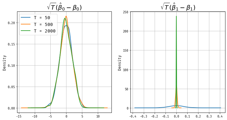
Let’s look at the distributions of \(\sqrt{T}(\hat\beta_1 - \beta_1)\) and \(\sqrt{T}(\hat\beta_2 - \beta_2)\)
A Monte Carlo
Some math
Facts:
\begin{eqnarray*} \sum_{t=1}^T 1 = T,\quad \sum_{t=1}^T t = T(T+1)/2, \quad\sum_{t=1}^T t^2 = T(T+1)(2T+1)/6. \end{eqnarray*}
(Assume \(u_t’s\) are independently distributed.)
\[ \frac{1}{T} \sum x_t x_t’ = \frac{1}{T} \left( \begin{array}{cc} \sum 1 & \sum t \\ \sum t & \sum t^2 \end{array} \right) \] are not convergent!
On the other hand
\[
\frac{1}{T^{\textcolor{red}{3}}} \sum x_t x_t’ \longrightarrow
\left( \begin{array}{cc} 0 & 0 \\ 0 & 1/3 \end{array} \right)
\]
which is singular and not invertible!
Message: Trends change the rate of convergence of estimators!
More on Rates of Convergence
It turns out that \(\hat{\beta}_{1,T}\) and \(\hat{\beta}_{2,T}\) have different asymptotic rates of convergence. In particular, we will learn faster about the slope of the trend line than the intercept.
To analyze the asymptotic behavior of the estimators we define the matrix \[ G_T = \left( \begin{array}{cc} 1 & 0 \\ 0 & T \end{array} \right). \] Note that the matrix is equivalent to its transpose, that is, \(G_T = G_T’\).
Asymptotic Distributions
We will analyze the following quantity \[ G_T(\hat{\beta}_T - \beta) = \left( \frac{1}{T} \sum G_T^{-1} x_t x_t’G_T^{-1} \right)^{-1} \left( \frac{1}{T}\sum G_T^{-1} x_t u_t \right). \] It can be easily verified that \[ \frac{1}{T} \sum G_T^{-1} x_t x_t’ G_T^{-1} = \frac{1}{T} \left( \begin{array}{cc} \sum 1 & \sum t/T \\ \sum t/T & \sum (t/T)^2 \end{array} \right) \longrightarrow Q, \] where \[ Q = \left( \begin{array}{cc} 1 & 1/2 \\ 1/2 & 1/3 \end{array} \right). \]
Standardization
The term \(\frac{1}{T} \sum G_T^{-1} x_t u_t\) has the components
\(\frac{1}{T} \sum u_t\) and \(\frac{1}{T} \sum (t/T) u_t\) which converge
in probability to zero based on the weak law of large numbers for non-identically
distributed random variables.
Note: Without the proper standardization \(\frac{1}{T} \sum t u_t\)
will not converge to its expected value of zero. The variance of the
random variable \(T u_T\) is getting larger and larger with sample size which
prohibits the convergence of the sample mean to its expectation. \(\Box\)
Results
Result: Suppose \[ y_t = \beta_1 + \beta_2 t + u_t, \quad u_t \sim iid(0,\sigma^2). \] Let \(\hat{\beta}_{i,T}\), \(i=1,2\) be the OLS estimators of the intercept and slope coefficient, respectively. Then
\begin{eqnarray} \hat{\beta}_{1,T} -\beta_1 & \stackrel{p}{\longrightarrow} & 0 \label{eq_rint}\\ T(\hat{\beta}_{2,T} - \beta_2) & \stackrel{p}{\longrightarrow} & 0 \label{eq_rslp}. \quad \Box \end{eqnarray}
CLT
I’m not going to show the details of proof for CLT, but
We use a CLT for independently but not identically distributed random variables (Liapounov)
Also, Cramer and Wold device that can be used to deduce the convergence of a random vector
based on the convergence of arbitrary linear combinations of its elements.
Result \[ y_t = \beta_1 + \beta_2 t + u_t, \quad u_t \sim iid(0,\sigma^2). \] Let \(\hat{\beta}_{i,T}\), \(i=1,2\) be the OLS estimators of the intercept and slope coefficient, respectively. The sampling distribution of the OLS estimators has the following large sample behavior \[ \sqrt{T} G_T (\hat{\beta}_T - \beta) \Longrightarrow {\cal N}(0,\sigma^2Q^{-1}) \]
Note
This is equivalent to \[ \left[ \begin{array}{c} \sqrt{T}(\hat{\beta}_{1,T} - \beta) \\ T^{3/2}(\hat{\beta}_{2,T} - \beta_2) \end{array} \right] \Longrightarrow {\cal N} \left( \left[ \begin{array}{c} 0 \\ 0 \end{array} \right], \sigma^2 \left[ \begin{array}{cc} 4 & -6 \\ -6 & 12 \end{array} \right] \right). \quad \Box \]
Having Said All this
When we consider the case where the variance is unknown:
\[ \hat \sigma^2 = \frac{1}{T-2}\sum(y_t - \hat\beta_1 - \hat\beta_2 t)^2 \]
Despite the fact that \(\beta_1\) and \(\beta_2\) have different asymptic rates of convergence, the t statistics still have \(N(0,1)\) limited distribution because the standard error estimates have offsetting behaviour.
OLS and Serial Dependence
\[ y_t = \beta t + u_t \] \(u_t\) are serially correlated, that is, \(\mathbb E[u_{t}u_{t-h}] \not= 0\) for some \(h \implies\) OLS not efficient.
Let’s look at example with \(MA(1)\) errors. \[ u_t = \epsilon_t + \theta \epsilon_{t-1}, \quad \epsilon_{t} \sim iid(0,\sigma^2_\epsilon). \] can verify
\begin{eqnarray} \mathbb E[u_t^2] & = & \mathbb E[(\epsilon_t + \theta \epsilon_{t-1})^2] = (1+\theta^2)\sigma^2_\epsilon \\ \mathbb E[u_tu_{t-1}] & = & \mathbb E[ (\epsilon_t + \theta \epsilon_{t-1})(\epsilon_{t-1} + \theta \epsilon_{t-2})] = \theta \sigma^2_\epsilon \\ \mathbb E[u_tu_{t-h}] & = & 0 \quad h > 1. \end{eqnarray}
The OLS estimator
\[ \hat{\beta}_T - \beta = \frac{\sum tu_t}{\sum t^2}. \] To find the limiting distribution, note that \[ \frac{1}{T^3} \sum_{t=1}^T t^2 = \frac{T(T+1)(2T+1)}{6T} \longrightarrow \frac{1}{3}. \]
Numerator
The numerator can be manipulated as follows
\begin{eqnarray} \sum t u_t & = & \sum t(\epsilon_t + \theta \epsilon_{t-1}) \nonumber \\ & = & \begin{array}{ccccc} 0 & +\epsilon_1 & +2\epsilon_2 & + 3\epsilon_3 & + \ldots \\ +\theta \epsilon_0 & + 2 \theta \epsilon_1 & + 3 \theta \epsilon_2 & + 4 \theta \epsilon_3 & + \ldots \end{array} \nonumber \\ & = & \sum_{t=1}^{T-1} (t + \theta(t+1)) \epsilon_t \; + \theta \epsilon_0 + T \epsilon_T \nonumber \\ & = & \sum_{t=1}^{T-1} (1+\theta) t \epsilon_t + \sum_{t=1}^{T-1} \theta \epsilon_t + \theta \epsilon_0 + T \epsilon_T \nonumber \\ & = & \sum_{t=1}^T (1+\theta) t \epsilon_t \underbrace{ - \theta T \epsilon_T + \theta \sum_{t=1}^T \epsilon_{t-1} }_{\mbox{asymp. negligible}}. \end{eqnarray}
OLS, Continued
After standardization by \(T^{-3/2}\) we obtain
\begin{eqnarray*} T^{-3/2} \sum tu_t = \frac{1}{\sqrt{T}} (1+\theta) \sum_{t=1}^T (t/T) \epsilon_t - \frac{1}{\sqrt{T}} \theta \epsilon_T + \frac{\theta}{T} \frac{1}{\sqrt{T}} \sum_{t=1}^T \epsilon_{t-1}. \end{eqnarray*}
- First term obeys CLT
- Second Term goes to zero
- Third Term goes to zero
Thus , \[ T^{3/2}( \hat{\beta}_T - \beta) \Longrightarrow \big(0,3\sigma^2_\epsilon (1+\theta)^2 \big). \]
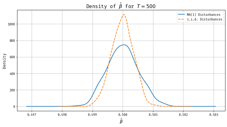
Remark
Consider the following model with \(iid\) disturbances \[ y_t = \beta t + u_t, \quad u_t \sim iid(0,\sigma_\epsilon^2(1+\theta^2)). \] The unconditional variance of the disturbances is the same as in the model with moving average disturbances. It can be verified that
\[ T^{3/2}( \hat{\beta}_T - \beta) \Longrightarrow \big(0,3\sigma^2_\epsilon (1+\theta^2) \big). \]
If \(\theta\) is positive then the limit variance of the OLS estimator in the
model with \(iid\) disturbances is smaller than in the trend model with moving
average disturbances.
Positive serial correlated data are less informative than \(iid\) data.
Sampling Distributions
Stochastic Trends
Stochastic Trends
We looked at stationary model and deterministic trend models so far.
Now we will examine univariate models with a stochastic trend of the form
\[ y_t = \phi_0 + y_{t-1} + \epsilon_t \quad \epsilon_t \sim iid(0,\sigma^2) \]
This particular model is called a random walk with drift.
The variable \(y_t\) is said to be integrated of order one.
Cointegration
Moreover, we will consider bivariate models with a common stochastic trend
\begin{eqnarray} y_{1,t} & = & \gamma y_{2,t} + u_{1,t} \\ y_{2,t} & = & y_{2,t-1} + u_{2,t} \end{eqnarray}
where \([u_{1,t}, u_{2,t}]’ \sim iid(0,\Omega)\). Both \(y_{1,t}\) and \(y_{2,t}\) have a stochastic trend. However, there exists a linear combination of \(y_{1,t}\) and \(y_{2,t}\), namely, \[ y_{1,t} - \gamma y_{2,t} = u_t \] that is stationary. Therefore, \(y_{1,t}\) and \(y_{2,t}\) are called cointegrated.
Background
In the late 80s and early 90s, this was a super hot research area.
- Dickey and Fuller (1979) examined the sampling distribution of estimators for autoregressive time series with a unit root and provided tables with critical values for unit root tests.
- In Phillips (1986) and (1987) published two papers on spurious regression and time series regressions with a unit root that employ the mathematical theory of convergence of probability measures for metric spaces. This marks a ``technological breakthrough’’ and the field started to grow at an exponential rate thereafter.
Three Choices
Consider the first order autoregressive model with mean zero: \[ y_t = \phi y_{t-1} + \epsilon_t, \quad \epsilon_t \sim iid{\cal N}(0,\sigma^2) \] Three cases
\(|\phi|<1\): stationarity! we talked about this last week
\(|\phi|>1\): explosive! We will not analyze explosive processes in this course.
\(|\phi|=1\). This is the unit root and will be the focus of this
part of the lecture. If \(\phi=1\) then the AR(1) model simplifies to
\[ y_t = y_{t-1} + \epsilon_t \]
With \(\Delta=1-L\), we have \(\Delta y_t = \epsilon_t\) form a stationary process, the random walk is called integrated of order one, denoted by \(I(1)\).
Difference b/w Stationary AR and Unit Root
Suppose that the AR process is initialized by \(y_0 \sim {\cal N}(0,1)\). Then \(y_t\) can be expressed as
\[ y_t = \phi^{t} y_0 + \sum_{\tau=1}^t \phi^{\tau -1} \epsilon_{t+1-\tau} \]
- The unconditional mean of \(y_t\) is given by
\[ \mathbb E[y_t] = \phi^{t-1} \mathbb E[y_0] + \sum_{\tau=1}^t \phi^{\tau -1} \mathbb E[\epsilon_\tau] = 0 \]
Differences, continued
The unconditional variance is \(y_t\) is given by
\begin{eqnarray} var[y_t] & = & \phi^{2(t-1)} var[y_0] + \sum_{\tau=1}^t \phi^{2(\tau-1)} var[\epsilon_\tau] \\ & = & \phi^{2(t-1)} var[y_0] + \sigma^2 \sum_{\tau=1}^t \phi^{2(\tau-1)} \nonumber \\ & = & \left\{ \begin{array}{lclcl} \phi^{2(t-1)} var[y_0] + \sigma^2 \frac{1 - \phi^{2t}}{1 - \phi^2} & \longrightarrow & \frac{\sigma^2}{1-\phi^2} & \mbox{if} & |\phi| < 1 \\ var[y_0] + \sigma^2 t & \longrightarrow & \infty & \mbox{if} & |\phi| =1 \end{array} \right. \nonumber \end{eqnarray}
as \(t \rightarrow \infty\).
Differences, continued
The conditional expectation of \(y_{t}\) given \(y_0\) is
\begin{eqnarray*} \mathbb E[y_{t}|y_0] = \phi^{\tau-1} y_0 \longrightarrow \left\{ \begin{array}{lcl} 0 & \mbox{if} & |\phi| < 1 \\ y_0 & \mbox{if} & \phi = 1 \end{array} \right\} \end{eqnarray*}
as \(t \rightarrow \infty\).
In the unit root case, the best prediction of future \(y_{t}\) is the initial \(y_0\) at all horizons, that is, ``no change’'.
In the stationary case, the conditional expectation converges to the unconditional mean. For this reason, stationary processes are also called ``mean reverting’'.
Result
Stationary and unit root processes differ in their behavior over long time horizons.
Suppose that \(\sigma^2=1\), and \(y_0=1\). Then the conditional mean and
variance of a process \(y_t\) with \(\phi = 0.995\) is given by
| Horizon \(t\) | 1 | 2 | 5 | 10 | 20 | 50 | 100 |
|---|---|---|---|---|---|---|---|
| \(\mathbb E[y_t\mid y_0]\) | 0.995 | 0.990 | 0.975 | 0.951 | 0.905 | 0.778 | 0.606 |
| \(\mathbb V[y_t \mid y_0]\) | 1.000 | 1.990 | 4.901 | 9.563 | 18.21 | 39.52 | 63.46 |
If interestered in long run predictions, very important to distinguish these two cases.
But note: long run predictions face serious extrapolation problem.
Frequentist Approach
To get a unit root test of the null hypothesis \(H_0: \phi = 1\), we have to find the sampling distribution of a suitable test statistic such as the \(t\) ratio \[ \frac{\hat{\phi}_T -1}{\sqrt{ \sigma^2 / \sum y_{t-1}^2 }} \] Under the generating mechanism \[ y_t = \phi_0 + y_{t-1} + \epsilon_t, \quad iid(0,\sigma^2) \] For stationary processes used a variety of WLLN and CLTs, unfortunately, these don’t apply.
Heuristic Overview of Asymptotics
Assume that \(\phi_0 = 0\), \(\sigma = 1\), and \(y_0 = 0\). Thus, the process \(y_t\) can be represented as \[ y_T = \sum_{t=1}^T \epsilon_t \] Summations will range from \(t=1\) to \(T\) unless stated otherwise. The central limit theorem for \(iid\) random variables implies \[ \frac{y_T}{\sqrt{T} } = \frac{1}{\sqrt{T}} \sum \epsilon_t \Longrightarrow {\cal N}(0,1) \] This suggests that \[ \frac{1}{T} \sum y_t = \frac{1}{\sqrt{T}} \sum \left[ \sqrt{ \frac{t}{T} } \frac{1}{\sqrt{t}} \sum_{\tau =1}^t \epsilon_\tau \right] \] will not converge to a constant in probability but instead to a random variable.
Need a more elegant approach!
A Twist on our framework
We used \(T = \{0, \pm 1, \pm 2, \ldots\}\).
Consider \(S = [0,1]\). Consider random elements \(W(s)\) that correspond to functions this interval.
We will place some probability \(Q\) on these functions and show that \(Q\) can be helpful in the approximation of the distribution of \(\sum y_t\)
Defining probability distributions on function spaces is a pain.
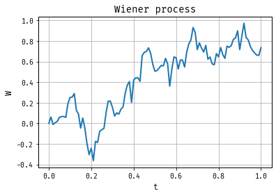
Wiener Measure
Let \({\cal C}\) be the space of continuous functions on the interval \([0,1]\).
We will define a probability distribution for the function space \({\cal C}\).
This probability distribution is called ``Wiener measure’'.
Whenever we draw an element from the probability space we obtain a function \(W(s)\), \(s \in [0,1]\). Let \(Q[ \cdot ]\) denote the expectation operator under the Wiener measure.
Properties of \(W(s)\)
- If we repeatedly draw functions under the Wiener measure and evaluate these functions at a particular value \(s = s’\), then \[ Q[ \{ W(s’) \le w \} ] = \frac{1}{\sqrt{2\pi s’}} \int_{-\infty}^{w} e^{- u^2/2s’} du\] that is, \[ W(s’) \sim {\cal N}(0,s’) \] If \(s’=0\) then the equations is interpreted to mean \(Q[\{W(0)=0 \}] = 1\). Thus \(W(0) = 0\) with probability one.
Properties of \(W(s)\)
- The random function \(W(s)\) has independent increments. If \[ 0 \le s_1 \le s_2 \le \ldots \le s_k \le 1 \] Then the random variables \[ W(s_2) - W(s_1), \; W(s_3) - W(s_2)\; \ldots , \; W(s_k) - W(s_{k-1}) \] are independent.
- The random function \(W(s)\) is continuous on \(s \in [0,1]\). Otherwise, contradiction.
More of \(W(s)\)
It can be shown that there indeed exists a probability distribution on \({\cal C}\) with these properties.
Rougly speaking, the Wiener measure is to the theory of stochastic processes, what the normal distribution is to the theory related to real valued random variables.
Note: \(W(1) \sim {\cal N}(0,1)\).
Relating this back to our discrete processes
Define the partial sum process \[ Y_T(s) = \frac{1}{\sqrt{T}} \sum \{ t \le \lfloor Ts \rfloor \} \epsilon_t \] where \(\lfloor x \rfloor\) denotes the integer part of \(x\). Since we assumed that \(\epsilon_t \sim iid(0,1)\), the partial sum process is a random step function.
Interpolation:
\begin{eqnarray*} \bar{Y}_T(s) = \frac{1}{\sqrt{T}} \sum \{ t \le \lfloor Ts \rfloor \} \epsilon_t + (Ts - \lfloor Ts \rfloor ) \epsilon_{\lfloor Ts \rfloor + 1} / \sqrt{T} \end{eqnarray*}
Two ways to randomly generate continuous functions
Draw a function \(W(s)\) from the Wiener distribution. We did not examine how to do the sampling in practice, but since the Wiener distribution is well-defined, it is theoretically possible.
Generate a sequence \(\epsilon_1, \ldots, \epsilon_T\), where \(\epsilon_t \sim iid(0,1)\) and compute \(\bar{Y}_T(s)\).
As \(T\longrightarrow\infty\), these are basically the same.
Functional CLT: Let \(\epsilon_t \sim iid(0,\sigma^2)\). Then
\begin{eqnarray*} Y_T(s) = \frac{1}{\sigma \sqrt{T} } \sum_{t=1}^T \{ t \le \lfloor Ts \rfloor \} \epsilon_t \Longrightarrow W(s) \quad \Box \end{eqnarray*}
Simulation of Wiener Process
The upshot
The sum \[ \frac{1}{T} \sum y_{t-1} \epsilon_t \] convergences to a stochastic integral; i.e.,
Suppose that \(y_t = y_{t-1} + \epsilon_t\), where \(\epsilon_t \sim iid(0,\sigma^2)\) and \(y_0=0\). Then \[ \frac{1}{\sigma^2 T} \sum y_{t-1} \epsilon_t \Longrightarrow \int W(s) dW(s) \] where \(W(s)\) denotes a standard Wiener process.
we can use this to develop tests!
Theorem
Suppose that \(y_t = \phi y_{t-1} + \epsilon_t\), where \(\epsilon_t \sim iid(0,\sigma^2)\), \(\phi=1\), and \(y_0=0\). The sampling distribution of the OLS estimator \(\hat{\phi}_T\) of the autoregressive parameter \(\phi=1\) and the sampling distribution of the corresponding \(t\)-statistic have the following asymptotic approximations
\begin{eqnarray} z(\hat{\phi}_T) & \Longrightarrow & \frac{\frac{1}{2} ( W(1)^2 -1 ) }{ \int_0^1 W(s)^2 ds } \\ t(\hat{\phi}_T) & \Longrightarrow & \frac{\frac{1}{2} ( W(1)^2 -1 ) }{ \left[ \int_0^1 W(s)^2 ds \right]^{1/2} } \end{eqnarray}
where \(W(s)\) denotes a standard Wiener process. \(\Box\)
How These Sampling Distributions look
import numpy as np
import matplotlib.pyplot as plt
from statsmodels.tsa.ar_model import AutoReg
from scipy.stats import norm

# Parameters
T = 5000  # Length of time series
N_sim = 2000  # Number of simulations
phi_values = [1, 0.95]

# Function to simulate AR(1) process and estimate
def simulate_and_estimate(phi, T, N_sim):
    estimates = np.zeros(N_sim)
    for i in range(N_sim):
        y = np.zeros(T)
        for t in range(1, T):
            y[t] = phi * y[t-1] + np.random.normal()
        model = AutoReg(y, lags=1, trend='n').fit()
        estimates[i] = (model.params[-1] - phi) / model.bse[-1]
    return estimates

# Function to simulate the Wiener process distribution
def simulate_wiener(phi, T, N_sim):
    np.random.seed(42)
    estimates = np.zeros(N_sim)
    for i in range(N_sim):
        W = np.random.normal(size=T).cumsum() / np.sqrt(T)
        W1 = W[-1]
        integral_W2 = np.sum(W**2) / T
        estimates[i] = 0.5 * (W1**2 - 1) / integral_W2**0.5
    return estimates

# Run simulations
empirical_estimates = {str(phi): simulate_and_estimate(phi, T, N_sim) for phi in phi_values}
phi_1_distribution = simulate_wiener(1, T, N_sim)

# Plot results
plt.figure(figsize=(14, 6))

# Plot for phi = 1
plt.subplot(1, 2, 1)
plt.hist(empirical_estimates['1'], bins=30, density=True, alpha=0.7, label='Empirical for $\phi=1$')
# kde for the theoretical distribution from draws phi_1_distribution
from scipy.stats import gaussian_kde
kde = gaussian_kde(phi_1_distribution)
x = np.linspace(-3, 3, 1000)
plt.plot(x, kde(x), label='Asymptotic for $\phi=1$', linestyle='--')
plt.title(r'Sampling Distribution for $\phi=1$')
plt.xlabel(r'$\hat{\phi}$')
plt.grid()
plt.legend()

# Plot for phi = 0.95
plt.subplot(1, 2, 2)
plt.hist(empirical_estimates['0.95'], bins=30, density=True, alpha=0.7, label='Empirical for $\phi=0.95$')
x = np.linspace(-3, 3, 1000)
plt.plot(x, norm.pdf(x, loc=0, scale=1), label='Theoretical N(0.95, var)', linestyle='--')
plt.title(r'Sampling Distribution for $\phi=0.95$')
plt.xlabel(r'$\hat{\phi}$')
plt.grid()
plt.legend()

plt.tight_layout()
plt.show()
Back to Nelson and Plosser (1982)
log Real GNP: estimated autocorrelation functions of the level and deviations from the time trend
Looks good, but can give misleading results when the underlying series is integrated. \[ y_t = \mu + \phi_1 y_{t-1} + \gamma t + \sum_{k=1}^K \phi_{\Delta k}\Delta y_{t-k} + u_t. \] want to test \(\phi_1 = 1\).
Results
- t-stat is the conventional t-stat!
- Dickey-Fulley 5 percent critial value is about \(-3.5\).
Thus, one cannot reject the null that real GNP is well described by a unit root process!
Cointegration
Back to Our Model
We will now analyze a simple bivariate system of cointegrated processes. Consider the model
\begin{eqnarray} y_{1,t} & = & \gamma y_{2,t} + u_{1,t} \\ y_{2,t} & = & y_{2,t-1} + u_{2,t} \end{eqnarray}
where \([u_{1,t},u_{2,t}]’ \sim iid(0,\Omega)\).
Clearly, \(y_{2,t}\) is a random walk. Moreover, it can be easily verified that \(y_{1,t}\) follows a unit root process.
\begin{eqnarray} y_{1,t} - y_{1,t-1} = \gamma (y_{2,t} - y_{2,t-1}) + u_{1,t} - u_{1,t-1} \end{eqnarray}
Therefore,
\begin{eqnarray} y_{1,t} = y_{1,t-1} + \gamma u_{2,t} + u_{1,t} - u_{1,t-1} \end{eqnarray}
Thus, both \(y_{1,t}\) and \(y_{2,t}\) are integrated processes.
Model Continued
However, the linear combination
\begin{eqnarray} [1,\; -\gamma] \left[ \begin{array}{c} y_{1,t} \\ y_{2,t} \end{array} \right] = y_{1,t} - \gamma y_{2,t} = u_{1,t} \end{eqnarray}
is stationary. Therefore, \(y_{1,t}\) and \(y_{2,t}\) are cointegrated.
The vector \([1,-\gamma]’\) is called the cointegrating vector.
Note that the cointegrating vector is only unique up to normalization.
Rewriting the Model
The model can be rewritten as a VAR(1)
\begin{eqnarray} y_t = \Phi_1 y_{t-1} + \epsilon_t \end{eqnarray}
The elements of the matrix \(\Phi_1\) and the definition of \(\epsilon_t\) is given by
\begin{eqnarray} \left[ \begin{array}{c} y_{1,t} \\ y_{2,t} \end{array} \right] = \left[ \begin{array}{cc} 0 & \gamma \\ 0 & 1 \end{array} \right] \left[ \begin{array}{c} y_{1,t-1} \\ y_{2,t-1} \end{array} \right] + \left[ \begin{array}{c} u_{1,t} + \gamma u_{2,t} \\ u_{2,t} \end{array} \right] \end{eqnarray}
The matrix \(\Phi_1\) is of reduced rank in this example of
cointegration. More generally cointegrated system can be casted in
the form of a vector autoregression in levels of \(y_t\).
Although both \(y_{1,t}\) and \(y_{2,t}\) follow univariate random walks,
the cointegrated system cannot be expressed as a vector autoregression
in differences \([ \Delta y_{1,t}, \Delta y_{2,t} ]’\). Consider
\begin{eqnarray} \left[ \begin{array}{c} \Delta y_{1,t} \\ \Delta y_{2,t} \end{array} \right] = \left[ \begin{array}{cc} 1-L & \gamma L \\ 0 & 1 \end{array} \right] \left[ \begin{array}{c} u_{1,t} \\ u_{2,t} \end{array} \right] = \Theta(L) u_t \end{eqnarray}
Since \(|\Theta(1)|=0\) the moving average polynomial is not invertible and no finite order VAR could describe \(\Delta y_t\).
VECM
The cointegrated model can be written in the so-called vector error correction model (VECM) form:
\begin{eqnarray} \left[ \begin{array}{c} \Delta y_{1,t} \\ \Delta y_{2,t} \end{array} \right] = \left[ \begin{array}{c} -1 \\ 0 \end{array} \right] \left( \left[ \begin{array}{cc} 1 & - \gamma \end{array} \right] \left[ \begin{array}{c} y_{1,t-1} \\ y_{2,t-1} \end{array} \right] \right) + \left[ \begin{array}{c} u_{1,t} + \gamma u_{2,t} \\ u_{2,t} \end{array} \right] \end{eqnarray}
The term
\begin{eqnarray} \left( \left[ \begin{array}{cc} 1 & - \gamma \end{array} \right] \left[ \begin{array}{c} y_{1,t-1} \\ y_{2,t-1} \end{array} \right] \right) = y_{1,t-1} - \gamma y_{2,t-1} \end{eqnarray}
is called error correction term. In economic models it often reflects a long-run equilibrium relationship such as a constant ratio of consumption and output. If the economy is out of equilibrium in period \(t-1\), that is, \(y_{1,t-1} - \gamma y_{2,t-1} \not= 0\), then the economy adjusts toward its long-run equilibrium and \(\EE_{t-1}[\Delta y_{t}] \not= 0\). If the ``true’’ cointegrating vector is known, then both the left-hand-side variables and the error correction term are stationary.