Lecture X Bayesian Nonparametrics

Introduction

What are Bayesian Nonparametrics?

We start with data \(y_1, \ldots, y_n \) drawn from a distribution \(G\).

A ‘statistical model’ \(g\) is a pdf of \(G\), where \(g \in \mathcal{G} = \{g_\theta: \theta \in \Theta\}.\)

If \(\theta\) is finite, we are into the realm of parametric statistics.

If \(\theta\) is infinite, we are into the realm of nonparametric statistics.

Bayesian nonparametrics complete the above probability model with a prior distribution on the infinite-dimensional parameter \(\theta\).

Dirichlet Process

Density Estimation

Density estimation: given an observed sample, infer underlying density. \[ y_i | G \overset{iid}{\sim} G, \quad i = 1, \ldots, n. \] Bayesian inference: complete the model with a prior probability model \(\pi\) for the unknown parameter \(G\).

We need a probability model for the infinite dimensional parameter \(G\), a BNP prior

Dirichlet Process

A Dirichlet Process (DP) is a probability distribution over probability distributions, first introduced in (Ferguson, Thomas S., 1973).

It is parameterized by a base measure \(G_0\) and a concentration parameter \(\alpha\).

Formally, given a base measure \(G_0\) and a concentration parameter \(\alpha\), a random distribution \(G\) is said to be distributed according to a Dirichlet Process, denoted as \(G \sim DP(\alpha, G_0)\), if for any finite partition \(\{A_i\}\) of the sample space: \[ (G(A_1), …, G(A_n)) \sim Dir(\alpha G_0(A_1), …, \alpha G_n(A_n)) \] Kolmogorov’s consistency theorem guarantees that there exists a random probability measure \(G\) such that the above property holds.

Definition of a Dirichlet Random Variable

The Dirichlet distribution is a probability distribution over probability distributions in a finite-dimensional simplex.

Let \(X = (X_1, …, X_n)\) be a random vector that follows a Dirichlet distribution with parameters \(\alpha_1, …, \alpha_n\), such that: \[ X \sim Dir(\alpha_1, …, \alpha_n) \] Then, the joint probability density function of X is given by: \[ p(X) = \frac{1}{B(\boldsymbol{\alpha})} \prod_{i=1}^{n} X_i^{\alpha_i - 1}, \] where \(B(\boldsymbol{\alpha})\) is the multinomial Beta function, defined as: \[ B(\boldsymbol{\alpha}) = \frac{\prod_{i=1}^{n} \Gamma(\alpha_i)}{\Gamma(\sum_{i=1}^{n} \alpha_i)} \] The Dirichlet Process can be seen as an extension of the Dirichlet distribution to an infinite number of dimensions.

Some Properties of the Dirichlet Process

Consider the sample space \(\{B, B^c\}\). We have:

1. G has the same support as \(G_0\). That is, \(Pr[G(B)>0] = 1 \iff G_0(B) > 0\). This is because \(G(B) \sim Dir(\alpha G_0(B), \alpha G_0(B^c))\).
2. For all \(B\), \(\mathbb E[G(B)] = G_0(B)\). This is because \(\mathbb E[G(B)] = \frac{\alpha G_0(B)}{\alpha G_0(B) + \alpha G_0(B^c)} = G_0(B)\).
3. For all \(B\), \(\mathbb V[G(B)] = \frac{G_0(B)(1-G_0(B))}{1+\alpha}\).

Constructing DP: Stick Breaking

(Sethuraman, Jayaram, 1994) showed that the Dirichlet Process can be constructed using a stick-breaking process.

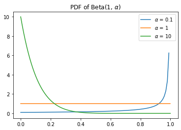
Imagine you have a stick of length 1, and you break it at a random point \(V_1\), such that \(V_1 \sim Beta(1, \alpha)\).

You then take the remaining stick of length \(1 - V_1\) and break it at a random point \(V_2\), such that \(V_2 \sim Beta(1, \alpha)\).

The total length of the second stick is \(W_2 = (1 - V_1)V_2\) (and the first stick is length \(V_1\)).

If we repeat this \(n\) times, we’re left with a set of realization of random variables \(W_1, W_2, …\), such that \(\sum_{i=1}^{}^n W_i = 1\).

More stick breaking:

To complete a construction of the DP, we draw \(\theta_i \sim G_0\) for \(i = 1, \ldots, n\).

We are left with the (discrete) random probability measure: \[ G(\cdot) = \sum^n_{i=1} W_i \delta_{\theta_i}(\cdot), \mbox{ with } \delta_{\theta_i}(\cdot) \sim G_0. \] As \(n\) becomes large, \(G \sim DP(\alpha, G_0)\).

How does this work?

The Role of \(\alpha\)

Thinking this through

The concentration parameter \(\alpha\) controls the amount of mass that is assigned to the atoms \(\theta_i\).

If \(\alpha\) is very large, then all of the sticks will be small and the resulting distribution will “look” a lot like the base measure \(G_0\).

If \(\alpha\) is very small, then the first few sticks will be large, and the resulting distribution will be a mixture of the base measure \(G_0\) and the atoms \(\theta_i\).

Varying \(\alpha\)

Let’s let \(\alpha\) vary in \(\{1, 20, 100\}\) and see how the resulting distributions change.

We’ll use a base measure \(G_0\) that is a normal distribution with mean 0 and variance 1.

We’ll take 1000 draws from the DP and plot density estimates of the resulting distributions.

---------------------------------------------------------------------------
NameError                                 Traceback (most recent call last)
<ipython-input-2-e320bd606115> in <module>
     28     ax[i].set_title(r'$\alpha$ = {}'.format(a))
     29 
---> 30     ax[i].plot(x, norm.pdf(x), color='black', linewidth=3)
     31     ax[i].set_title(r'$\alpha$ = {}'.format(a))
     32     ax[i].set_xlim(-3, 3)

NameError: name 'norm' is not defined

DP as a Prior (and Posterior)

The DP is used as a prior for the distribution of the data, and the posterior distribution of the DP is also a DP.

Let \(X_1, \ldots, X_n\) be an (iid) random sample from a distribution \(F\).

Let \(G\) be a DP prior with base measure \(G_0\) and concentration parameter \(\alpha\).

Then the posterior distribution of \(G\) given \(X_1, \ldots, X_n\) is: \[ G \mid X_1, \ldots, X_n \sim DP\left(\alpha + n, \frac{\alpha}{\alpha + n} G_0 + \frac{n}{\alpha + n} \frac{1}{n} \sum_{i=1}^n \delta_{X_i} \right). \]

An Example

Let’s take a look at an example of the DP as a prior and posterior.

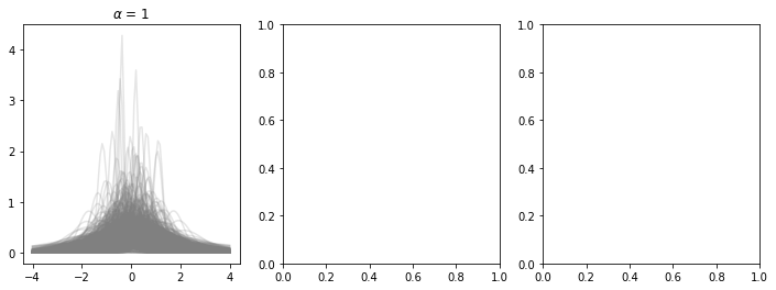
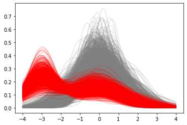
We’ll use a base measure \(G_0\) that is a normal distribution with mean 0 and variance 1. We’ll set \(\alpha = 10\).

Suppose we observe 10 data points from a normal distribution with mean \(\mu = -3\) and variance \(\sigma^2 = 0.1\).

We’ll take 100 draws from the DP prior and posterior and plot density estimates of the resulting distributions.

The Prior and Posterior

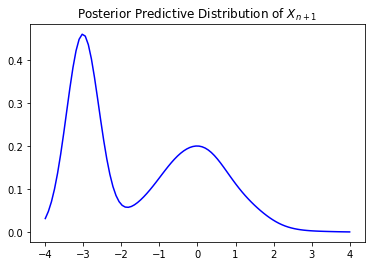
Posterior Predictive Distribution

The posterior predictive distribution is the distribution of a new observation given the data.

Then the posterior predictive distribution of \(X_{n+1}\) given \(X_1, \ldots, X_n\) is: \[ X_{n+1} \mid X_1, \ldots, X_n \sim \int F(\cdot) \, dG \sim \frac{\alpha}{\alpha + n} G_0 + \frac{n}{\alpha + n} \frac{1}{n} \sum_{i=1}^n \delta_{X_i}. \] This is the mixture of the prior and the empirical distribution of the data.

We can draw from this distribution by drawing from the base measure and the empirical distribution and then choosing between them with probability \(\frac{\alpha}{\alpha + n}\) and \(\frac{n}{\alpha + n}\), respectively.

An Example

Let’s take a look at an example of the posterior predictive distribution of the earlier example.

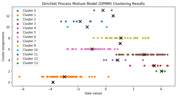
Dirichlet Process Mixtures (DPM)

The Dirichlet Process Mixture (DPM) is a Bayesian nonparametric model that uses the DP as a prior on the mixing distribution.

That is, suppose we believe that the data are generated from a mixture of distributions (e.g., a mixture of normals).

Then we can use the DP as a prior on the mixing distribution.

We don’t need to know the number of components in the mixture!

Reference: (Antoniak, Charles E, 1974)

An example

Suppose we have a (possibly infinite) mixture of normals with unknown mean and variance.

\[ \{\mu_k, \sigma_k^2\}_{k=1}^\infty \sim G, \quad G \sim \text{DP}(\alpha, G_0) \]

Our data is distributed as: \[ X_i \mid \mu_k, \sigma_k^2 \sim \mathcal{N}(\mu_k, \sigma_k^2) \]

We can estimate this model via a Gibbs sampler, see (Neal, Radford M, 2000) and (Escobar, Michael D and West, Mike, 1995).

DPM

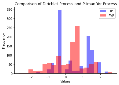
Extension: Pitman-Yor process

The DP is a special case of the Pitman-Yor process (PYP).

The PYP is parameterized by \(\alpha\), \(G_0\), and an additional parameter \(d \in [0, 1)\).

\(d\) has the interpretation of a “discount” parameter. (DP is the special case where \(d=0\).)

It’s best understood in the context of its stick-breaking construction.

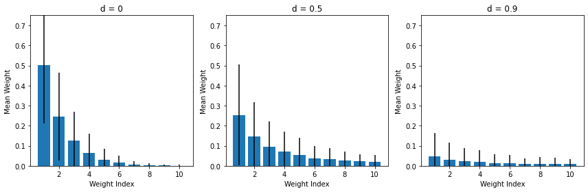
Stick-breaking for the PYP

The stick-breaking construction for the PYP is similar to that of the DP.

We are going to draw our stick lengths from a beta distribution, but with a twist.

For \(i=1,2,\ldots\), we draw from \(V_i \sim \mathcal B(1-d, \alpha + id)\) distribution.

For larger values of \(d\), the initial \(V_i\) are likely to

The role of \(d\)

PYP vs DP

Mean weights: 0.0100, std: 0.019
Mean weights: 0.0100, std: 0.007

Gaussian Process

Gaussian Process

A Gaussian Process (GP) is a collection of random variables, any finite number of which have a joint Gaussian distribution.

It is completely specified by its mean function \(m(x)\) and covariance function \(k(x, x’)\).

Formally: \(GP(m(x), k(x, x’))\) which can be used to model a distribution over functions \(f(x)\).

As long as the covariance function is “valid,” Kolmogorov’s consistency theorem guarantee’s such a process exists.

Properties

A GP is completely characterized by its mean and covariance functions.

The mean function defines the expected value of the function at any point. \[ m(x) = \mathbb{E}[f(x)] \] The covariance function defines the covariance between the function values at any two points. \[ k(x, x’) = \mathbb{E}[(f(x) - m(x))(f(x’) - m(x’))] \] A GP is stationary if its mean is constant and covariance function does not depend on the absolute input values but only on the relative distances.

A GP is isotropic if its covariance function depends only on the Euclidean distance between the input points.

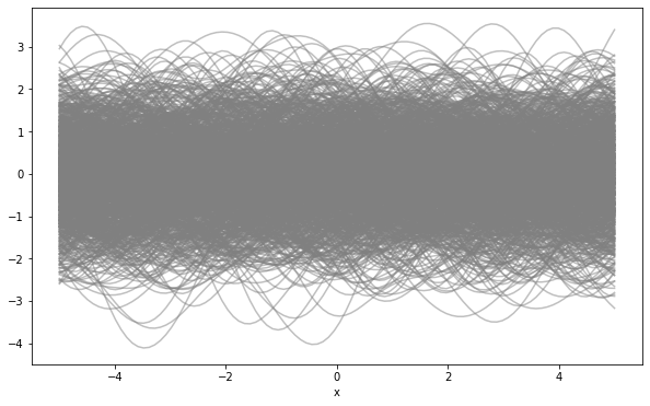
Simulating From a Gaussian Process

For example, we can use a zero mean function and a squared exponential covariance function. \[ m(x) = 0 \mbox{ and } k(x, x’) = \sigma^2 \exp\left(-\frac{(x - x’)^2}{2l^2}\right) \] where \(\sigma^2\) is the variance and \(l\) is the length scale.

Let’s set \(\sigma^2 = 1\) and \(l = 1\). Simulate as follows:

1. Make a grid of points \(\{x\}_{i=1}^n\) where we want to sample the function.
2. Compute the covariance matrix \(K\) for the grid points. \[ K = \left[k(x_i, x_j)\right]_{i,j=1}^n \]
3. Sample from a multivariate normal distribution with mean \(\mu = m(x) = 0\) and covariance \(K\).

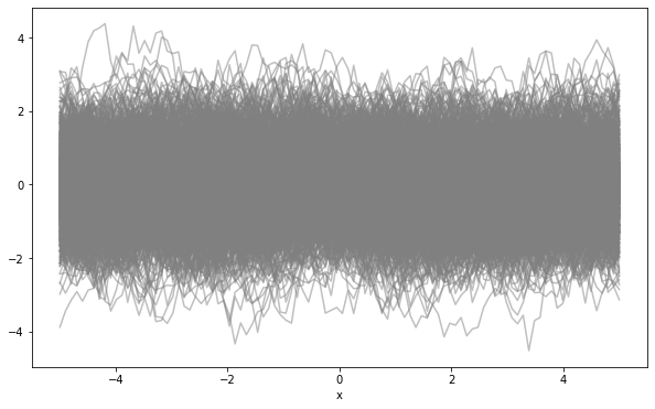
Example: 1000 Samples from a GP

Another example with a different covariance function

Posterior Inference

Suppose we have some data \(\{x_i, y_i\}_{i=1}^n\) and we want to infer the function \(f(x)\) that generated the data. We write: \[ y_i = f(x_i) + \epsilon_i, \quad \epsilon_i \overset{iid}{\sim} \mathcal{N}(0, \sigma^2) \] We can use a GP prior on \(f(x)\) and then use Bayes’ rule to compute the posterior distribution of \(f(x)\) given the data. Let \(Y = (y_1, \ldots, y_n)\) and \(X = (x_1, \ldots, x_n)\).

The posterior distribution of \(f(x)\) is also a GP with mean and covariance: \[ \overline m = m + K[K + \sigma^2 I]^{-1}(Y - m) \mbox{ and } \overline K = K - K[K + \sigma^2 I]^{-1}K \]

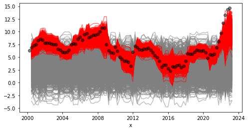
Example: GP Autoregression

Let \(x_t\) be a time series of year over year inflation rates.

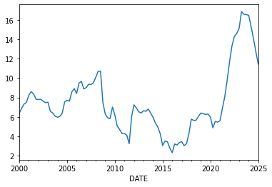
Example: GP Autoregression

Let’s use a GP to model the time series: \[ x_t = f(x_{t-1}) + \epsilon_t, \quad \epsilon_t \sim N(0, \sigma^2) \] We’ll use a GP prior with a squared exponential covariance function: \[ m(x) = 3 \mbox{ and } k(x, x’) = \kappa^2 \exp\left(-\frac{(x - x’)^2}{2l^2}\right). \]

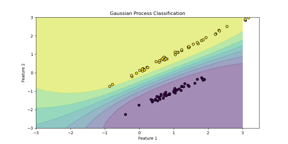
Classification: Gaussian Process Classification

• Gaussian Process Classification (GPC) is a nonparametric method for modeling the relationship between input variables and a categorical output variable.
• GPC extends the Gaussian Process framework to classification problems using a link function, such as the logistic or probit functions.

References

References

bibliographystyle:econometrica bibliography:/home/eherbst/Dropbox/ref/ref.bib

References

References

Antoniak, Charles E (1974). Mixtures of Dirichlet processes with applications to Bayesian nonparametric problems, JSTOR.

Escobar, Michael D and West, Mike (1995). Bayesian density estimation and inference using mixtures, Taylor \& Francis.

Ferguson, Thomas S. (1973). A Bayesian Analysis of Some Nonparametric Problems, Institute of Mathematical Statistics.

Neal, Radford M (2000). Markov chain sampling methods for Dirichlet process mixture models, Taylor \& Francis.

Sethuraman, Jayaram (1994). A constructive definition of Dirichlet priors, JSTOR.