Intro to Bayesian Analysis
Lecture Objectives:
Additional Readings:
Most presentations of econometrics focus on frequentist inference. That is, the properties of estimators and, more generally, inference procedures were examined from the perspective of repeated sampling experiments. The measures of accuracy and performance used to assess the statistical procedures were pre-experimental. However, many statisticians and econometricians believe that post-experimental reasoning should be used to assess inference procedures, wherein only the actual observation \(Y^T\) is relevant and not the other observations in the sample space that could have been observed,
Suppose \(Y_1\) and \(Y_2\) are independently and identically distributed and \[ P_\theta \{ Y_i = \theta-1 \} = \frac{1}{2}, \quad P_\theta \{ Y_i = \theta+1 \} = \frac{1}{2} \]
Consider the following confidence set for the parameter \(\theta\) in Example :
\begin{eqnarray*} C(Y_1,Y_2) = \left\{ \begin{array}{lcl} \frac{1}{2}(Y_1+Y_2) & \mbox{if} & Y_1 \not= Y_2 \\ Y_1 - 1 & \mbox{if} & Y_1 = Y_2 \end{array} \right. \end{eqnarray*}
\centering
\begin{tikzpicture}[scale=1.2] % Draw the grid \draw (0,0) rectangle (5,5); \draw (2.5,0) – (2.5,5); \draw (0,2.5) – (5,2.5);
% Label the axes
\node at (1.25,5.3) {\\(Y\_1 = \theta - 1\\)};
\node at (3.75,5.3) {\\(Y\_1 = \theta + 1\\)};
\node at (-1.0,1.25) {\\(Y\_2 = \theta - 1\\)};
\node at (-1.0,3.75) {\\(Y\_2 = \theta + 1\\)};

% Fill the boxes with colors
\filldraw[color=gray!30, border=black, pattern=north west lines] (0,2.5) rectangle (2.5,5);   % C = theta if Y1 = theta - 1, Y2 = theta - 1
\filldraw[color=gray!30, border=black, pattern=north west lines] (2.5,0) rectangle (5,2.5);   % C = theta if Y1 = theta + 1, Y2 = theta - 1
\filldraw[color=gray!30, border=black] (2.5,2.5) rectangle (5,5);   % C = theta if Y1 = theta + 1, Y2 = theta + 1
\filldraw[color=white, border=black] (0,0) rectangle (2.5,2.5);      % C not theta if Y1 = theta - 1, Y2 = theta + 1

% Draw patterned boxes (light cross hatching)
% \filldraw[pattern=north west lines,color=gray] (0, 2.5) rectangle (2.5, 5);
% Add confidence intervals
\node at (1.3,1.25) {\\(C(Y\_1,Y\_2) = \theta - 2\\)};
\node at (1.3,3.75) {\\(C(Y\_1,Y\_2) = \theta\\)};
\node at (3.75,1.25) {\\(C(Y\_1,Y\_2) = \theta\\)};
\node at (3.75,3.75) {\\(C(Y\_1,Y\_2) = \theta\\)};
\end{tikzpicture}
Figure 1 displays the confidence sets for the parameter \(\theta\) based on the realizations of \(Y_1\) and \(Y_2\). Note that each of the four boxes are equiprobable. In the case that \(Y_1 \ne Y_2\) (the cross hatched grey boxes), the confidence set contains the true value \(\theta\). When \(Y_1 = Y_2 = \theta + 1\) (the grey box in the upper left), the confidence set will again contain \(\theta\). But when \(Y_1 = Y_2 = \theta - 1\) (the white box in the lower left), the confidence will not contain \(\theta\). Thus, from a pre-experimental perspective \(C(Y_1,Y_2)\) is a 75% confidence interval. Since three of four (equally likely) boxes have realized confidence sets which contain \(\theta\), the the probability (under repeated sampling, conditional on \(\theta\)) that the confidence interval contains \(\theta\) 75%. But after seeing the realizations—the only way one can actually compute a confidence interval—we are a ``100% confident’’ that \(C(Y_1,Y_2)\) contains the ``true’’ \(\theta\) if \(Y_1 \not= Y_2\), whereas we are only ``50% percent’’ confident if \(Y_1 = Y_2\). This is the Bayesian post-experimental perspective, which emphasizes the role observed data. Does it make sense to report a pre-experimental measure of accuracy, when it is known to be misleading after seeing the data? The following conditionality principle appears quite reasonable.
We’ll begin with two core principles that will guide the discussion on inferential procedures. While both principles are widely accepted by statisticians, there is less consensus regarding their implications for inference.
Conditionality Principle: If an experiment is selected by some random mechanism independent of the unknown parameter \(\theta\), then only the experiment actually performed is relevant.
The conditionality principle highlights the importance of focusing soley on the realized data from an experiment, rather than on hypothetical scenarios that may have occurred but in fact did not. In the context of our Example , the realized values of \(Y_1\) and \(Y_2\) dictate the set of plausible values for the parameter \(\theta\).
The next principle focuses on the subject of parsimony in inference.
Sufficiency Principle: Consider an experiment to determine the value of an unknown parameter \(\theta\) and suppose that \({\cal S}(\cdot)\) is a sufficient statistic. If \({\cal S}(Y_1)={\cal S}(Y_2)\) then \(Y_1\) and \(Y_2\) contain the same evidence with respect to \(\theta\).
The concept of sufficiency in statistics relates features of data to information about the parameter of interest. A statistic is said to be sufficient for a parameter if the conditional distribution of the data, given the statistic, does not depend on the parameter. The combination of the quite reasonable Conditionality Principle and the Sufficiency Principle lead to the more controversial Likelihood Principle (see discussion in Robert (1994)).
Likelihood Principle: All the information about an unknown parameter \(\theta\) obtainable from an experiment is contained in the likelihood function of \(\theta\) given the data. Two likelihood functions for \(\theta\) (from the same or different experiments) contain the same information about \(\theta\) if they are proportional to one another.
Frequentist maximum-likelihood estimation and inference typically violates the Likelihood Principle (for a discussion see Robert (1994)) although it is based on likelihood functions. We will now study the Bayesian implementation of the Likelihood Principle.
A Bayes model consists of a parametric probability distribution for the data, which we will characterize by the density \(p(Y^T|\theta)\), and a prior distribution \(p(\theta)\). The density \(p(Y^T|\theta)\) interpreted as a function of \(\theta\) with fixed \(Y^T\) is the likelihood function. Data generation from such a model would consist of drawing a parameter \(\theta\) from the prior distribution \(p(\theta)\) and drawing a set of observations from the distribution \(p(Y^T|\theta’)\). The posterior distribution of the parameter \(\theta\), that is, the conditional distribution of \(\theta\) given \(Y_T\), can be obtained through Bayes theorem:
\begin{equation} p(\theta|Y^T) = \frac{ p(Y^T|\theta) p(\theta)}{ \int p(Y^T|\theta) p(\theta) d\theta} \end{equation}
One can interpret this formula as an inversion of probabilities. If you think of the parameter \(\theta\) as ``cause’’ and the data \(Y^T\) as ``effect’’, then the formula allows the calculation of the probability of a particular ``cause’’ given the observed ``effect’’ based on the probability of the ``effect’’ given the possible ``causes’'.
Unlike in the frequentist framework, the parameter \(\theta\) is regarded as a random variable. This does, however, not imply that Bayesians consider parameters to be determined in a random experiment. The calculus of probability is used to characterize the state of knowledge or the degree of beliefs of an individual with respect to events or quantities that have not (yet) been observed, and may not be observed, by that individual. The Bayesian approach prescribes consistency among the beliefs held by an individual, and their reasonable relation to any kind of objective data.
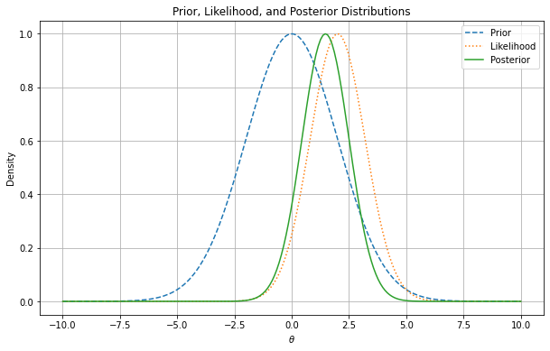
Figure shows an illustrative example of how prior beliefs, represented by the prior distribution, are updated by the data through the likelihood function to form the posterior distribution. The likelihood function is centered at 2, while the prior is centered at 0. The posterior distribution is a combination of the two, with the likelihood function having a stronger influence on the posterior distribution due to the data being more informative than the prior.
Any inference in a Bayesian framework is to some extent sensitive to the choice of prior distribution \(p(\theta)\). The prior reflects the initial state of mind of an individual and is therefore ``subjective’’. Many econometricians believe that the result of a scientific inquiry should not depend on the subjective beliefs of a researcher, and, are very skeptical of Bayesian methods. On the other hand, any econometric analysis and scientific investigation involves subjective choices by the researcher. (How did one decide which model to estimate?) The Bayesian approach simply makes these choices transparent. For the conclusions to be convincing among a group of individuals it is of course important to choose the prior carefully.
Bayesians have come up with several ideas on how to handle the delicate issue of priors. Box and Tiao (1973) advocated to report likelihood functions rather than posteriors and let the audience use their own priors. An alternative approach is to choose a ``reasonable’’ class of priors and demonstrate the conclusions are robust to changes of the prior distribution within this class. If there is additional information for a particular problem available it is usually good to incorporate this information into the prior to obtain more precise conclusions. The prior distribution could be interpreted as an augmentation of the data set. That is important for models that have many parameters relative to the number of observations that is available. Another approach are so-called “Objective Bayes” methods (see, for example, Berger (2006)) that seek to construct prior distributions in a systematic, non-subjective way, often based on principles of invariance—that is, prior distributions that remain unchanged under transformations of the data or parameters—or other criteria such as maximum entropy. These priors are typically non-informative or weakly informative priors, and are designed to minimize the influence of the prior on the posterior distribution while still adhering to Bayesian principle.
A prior distribution is called improper if
\begin{equation} \int_\Theta p(\theta)d\theta = \infty \end{equation}
Attempts to make priors non-informative, for instance, uniform on the real line, lead to improper priors. Maximum likelihood estimators can usually be interpreted as Bayes estimators that are based on an improper prior distribution. Bayes can still be used improper priors as long as the resulting posterior distribution is proper, meaning it integrates to one and can be interpreted as a valid probability distribution.
Introduction to Bayesian Statistics
We will denote the sample space by \({\cal Y}\) with elements \(Y^T\). A probability distribution \(P\) will be defined on the product space \(\Theta \otimes {\cal Y}\). The conditional distribution of \(\theta\) given \(Y^T\) is denoted by \(P_{Y^T}\), correspondingly, \(P_\theta\) denotes the conditional distribution of \(Y^T\) given \(\theta\). \(\mathbb E\), \(\mathbb E_{Y^T}\), and \(\mathbb E_\theta\) are the corresponding expectation operators. As before, we will use \(\{ x= x’ \}\) as indicator function that is one if \(x=x’\) and zero otherwise.
The parameter space is \(\Theta = \{ 0,1\}\), and the sample space is \({\cal Y}=\{0,1,2,3,4\}\).
| 0 | 1 | 2 | 3 | 4 | |
|---|---|---|---|---|---|
| \(P_{\theta=0}(Y)\) | .75 | .140 | .04 | .037 | .033 |
| \(P_{\theta=1}(Y)\) | .70 | .251 | .04 | .005 | .004 |
Suppose we consider \(\theta = 0\) and \(\theta=1\) as equally likely a priori. Moreover, suppose that the observed value is \(Y=1\). The marginal probability of \(Y=1\) is
\begin{multline} P \{ Y=1|\theta=0 \} P\{\theta=0\} +P \{ Y=1|\theta=1 \} P\{\theta=1\} = 0.140 \cdot 0.5 + 0.251 \cdot 0.5 = 0.1955 \end{multline}
The posterior probabilities for \(\theta\) being zero or one are
\begin{eqnarray*} P \{ \theta=0|Y=1 \} &=& \frac{ P \{Y=1|\theta=0 \} P\{ \theta = 0\} }{ P \{Y=1\} } = \frac{0.07}{0.1955} = 0.358 \\ P \{ \theta=1|Y=1 \} &=& \frac{ P\{Y=1|\theta=1 \} P\{ \theta = 1\} }{ P \{Y=1\} } = \frac{0.1255}{0.1955} = 0.642 \end{eqnarray*}
Thus, the observation \(Y=1\) provides evidence in favor of \(\theta = 1\).
Consider the linear regression model:
\begin{eqnarray} y_t = x_t’\theta + u_t, \quad u_t \stackrel{i.i.d.}{\sim}{\cal N}(0,1), \end{eqnarray}
where \(x_t\) and \(\theta\) have dimension \(k\). The regression model can be written as \(Y = X\theta + U\). We assume that \(X’X/T \stackrel{p}{\longrightarrow} Q_{XX}\) and \(X’Y \stackrel{p}{\longrightarrow} Q_{XY} = Q_{XX} \theta\).
The likelihood function is of the form
\begin{eqnarray} p(Y|X,\theta) = (2\pi)^{-T/2} \exp \left\{ -\frac12 (Y - X\theta)’(Y-X\theta) \right\}. \end{eqnarray}
Suppose the prior distribution is of the form
\begin{eqnarray} \theta \sim {\cal N} \bigg(0_{k \times 1},\tau^2 {\cal I}_{k \times k} \bigg) \end{eqnarray}
with density
\begin{eqnarray} p(\theta) = (2 \pi \tau^2 )^{-k/2} \exp \left\{ - \frac{1}{2 \tau^2} \theta’ \theta \right\} \end{eqnarray}
For small values of \(\tau\) the prior concentrates near zero, whereas for larger values of \(\tau\) it is more diffuse. According to Bayes Theorem the posterior distribution of \(\theta\) is proportional to the product of prior density and likelihood function
\begin{eqnarray} p(\theta | Y,X) \propto p(\theta) p(Y|X,\theta). \end{eqnarray}
The right-hand-side is given by
\begin{eqnarray} p(\theta) p(Y|X,\theta) \propto (2\pi)^{-\frac{T+k}{2}} \tau^{-k} \exp \bigg\{ -\frac{1}{2}[ Y’Y - \theta’X’Y - Y’X\theta - \theta’ X’X \theta \tau^{-2} \theta’\theta ] \bigg\}. \end{eqnarray}
The exponential term can be rewritten as follows
\begin{eqnarray} \lefteqn{ Y’Y - \theta’X’Y - Y’X\theta - \theta’ X’X \theta - \tau^{-2} \theta’\theta } \nonumber \\ &=& Y’Y - \theta’X’Y - Y’X\theta + \theta’(X’X + \tau^{-2} {\cal I}) \theta \\ &=& \bigg( \theta - (X’X + \tau^{-2} {\cal I})^{-1} X’Y \bigg)' \bigg(X’X + \tau^{-2} {\cal I} \bigg) \nonumber \\ && \bigg( \theta - (X’X + \tau^{-2} {\cal I})^{-1} X’Y \bigg) \nonumber \\ && + Y’Y - Y’X(X’X + \tau^{-2} {\cal I})^{-1}X’Y \nonumber. \end{eqnarray}
Thus, the exponential term is a quadratic function of \(\theta\). This information suffices to deduce that the posterior distribution of \(\theta\) must be a multivariate normal distribution
\begin{eqnarray} \theta |Y,X \sim {\cal N}( \tilde{\theta}_T, \tilde{V}_T ) \end{eqnarray}
with mean and covariance
\begin{eqnarray*} \tilde{\theta}_T &=& (X’X + \tau^{-2}{\cal I})^{-1} X’Y \\ \tilde{V}_T &=& (X’X + \tau^{-2}{\cal I})^{-1}. \end{eqnarray*}
The maximum likelihood estimator for this problem is \(\hat{\theta}_{mle} = (X’X)^{-1}X’Y\) and its asymptotic (frequentist) sampling variance is \(T^{-1} Q_{XX}^{-1}\).
The assumption that both likelihood function and prior are Gaussian made the derivation of the posterior relatively simple. The pair of prior and likelihood is called conjugate because it leads to a posterior distribution that is from the same family (multivariate normal) as the prior distribution.
As \(\tau \longrightarrow \infty\) the prior becomes more and more diffuse and the posterior distribution becomes more similar to the sampling distribution of \(\hat{\theta}_{mle}|\theta\):
\begin{eqnarray} \theta | Y,X \stackrel{approx}{\sim} {\cal N} \bigg( \hat{\theta}_{mle}, (X’X)^{-1} \bigg). \end{eqnarray}
If \(\tau \longrightarrow 0\) the prior becomes dogmatic and the sample information is dominated by the prior information. The posterior converges to a point mass that concentrates at \(\theta = 0\). In large samples (fixed \(\tau\), \(T \longrightarrow \infty\)) the effect of the prior becomes negligible and the sample information dominates
\begin{eqnarray} \theta |Y,X \stackrel{approx}{\sim} {\cal N} \bigg( \hat{\theta}_{mle}, T^{-1} Q_{XX}^{-1} \bigg). \quad \Box \end{eqnarray}
After having calculated posterior distributions we will now consider estimation and inference. In principle, all the information with respect to \(\theta\) is summarized in the posterior \(p(\theta|Y)\) and we could simply report the posterior density to our audience. However, in many situations our audience prefers results in terms of point estimates and confidence intervals, rather than in terms of a probability density. Moreover, we might be interested to answer questions of the form: do the data favor model \({\cal M}_1\) or \({\cal M}_2\)?
We will adopt a decision theoretic approach to develop the Bayesian estimation and inference procedures. In general, there is a decision rule \(\delta(Y^T)\) that maps observations into decisions, and a loss function \(L(\theta,\delta)\) according to which the decisions are evaluated.
\begin{eqnarray} \delta(Y^T) &:& {\cal Y} \mapsto {\cal D} \\ L(\theta,\delta) &:& \Theta \otimes {\cal D} \mapsto \RR^+ \end{eqnarray}
where \({\cal D}\) denotes the decision space. The goal is to find decisions that minimize the posterior expected loss \(\mathbb E_{Y^T} [ L(\theta, \delta(Y^T)) ]\). The expectation is taken conditional on the data \(x\), and integrates out the parameter \(\theta\). A decision theoretic treatment of estimation and inference can be found in Casella and Berger (2002), Lehmann (1997) Lehmann and Casella (1998), and Robert (1994).
Point Estimation
Suppose the goal is to construct a point estimate \(\delta(Y^T)\) of \(\theta\). It involves two steps:
- Find the posterior \(p(\theta|Y^T)\).
- Determine the optimal decision \(\delta(Y^T)\).
The optimal decision depends on the loss function \(L(\theta,\delta(Y^T))\).
Example 1, Continued: Consider the zero-one loss function
\begin{eqnarray} L(\theta,\delta) = \left\{ \begin{array}{l@{\quad}l} 0 & \delta = \theta \\ 1 & \delta \not= \theta \end{array} \right. \end{eqnarray}
The posterior expected loss is
\begin{eqnarray} \mathbb E_Y[L(\theta,\delta)] = 1 - \mathbb E_Y \{\theta = \delta\} \end{eqnarray}
The optimal decision rule is
\begin{eqnarray} \delta = \mbox{argmax}_{\theta’ \in \Theta} \; P_Y \{ \theta = \theta’\} \end{eqnarray}
that is, the point estimator under the zero-one loss is equal to the parameter value that has the highest posterior probability. We showed that
\begin{eqnarray*} P \{\theta = 0 |Y=1 \} &=& 0.358 \\ P \{\theta = 1 |Y=1 \} &=& 0.642 \end{eqnarray*}
Thus \(\delta(Y=1) = 1\). \(\Box\)
Example 2, Continued: The quadratic loss function is of the form
\begin{eqnarray} L(\theta,\delta) = (\theta - \delta)^2 \end{eqnarray}
The optimal decision rule is obtained by minimizing
\begin{eqnarray} \min_{\delta \in {\cal D}} \; \mathbb E_{Y^T} [(\theta - \delta)^2] \end{eqnarray}
It can be easily verified that the solution to the minimization problem is of the form \(\delta(Y^T) = \mathbb E_{Y^T} [\theta]\). Thus, the posterior mean \(\tilde{\theta}_T\) is the optimal point predictor under quadratic loss.
Suppose data are generated from the model \(y_t = x_t’\theta_0 + u_t\). Asymptotically the Bayes estimator converges to the ``true’’ parameter \(\theta_0\)
\begin{eqnarray} \tilde{\theta}_T &=& (X’X + \tau^{-2} {\cal I})^{-1} X’Y \\ &=& \theta_0 + \bigg( \frac{1}{T} X’X + \frac{1}{\tau^2 T}{\cal I} \bigg)^{-1} \bigg( \frac{1}{T} X’U \bigg) \nonumber \\ &\stackrel{p}{\longrightarrow} & \theta_0 \nonumber \end{eqnarray}
The disagreement between two Bayesians who have different priors will asymptotically vanish. \(\Box\)
Testing Theory
Consider the hypothesis test of \(H_0: \theta \in \Theta_0\) versus \(H_1: \theta \in \Theta_1\) where \(\Theta_1 = \Theta / \Theta_0\). Hypothesis testing can be interpreted as estimating the value of the indicator function \(\{\theta \in \Theta_0\}\). The decision space is 0 (``reject’’) and 1 (``accept’’). Consider the loss function
\begin{eqnarray} L(\theta,\delta) = \left\{ \begin{array}{l@{\quad}l@{\quad}l} 0 & \delta = \{\theta \in \Theta_0\} & \mbox{correct decision}\\ a_0 & \delta = 0, \; \theta \in \Theta_0 & \mbox{Type 1 error} \\ a_1 & \delta = 1, \; \theta \in \Theta_1 & \mbox{Type 2 error} \end{array} \right. \end{eqnarray}
Note that the parameters \(a_1\) and \(a_2\) are part of the econometricians preferences. The optimal decision rule is
\begin{eqnarray} \delta(Y^T) = \left\{ \begin{array}{l@{\quad}l} 1 & P_{Y^T}\{\theta \in \Theta_0\} \ge a_1/(a_0+a_1) \\ 0 & \mbox{otherwise} \end{array} \right. \end{eqnarray}
This can be easily verified. The expected loss is
\begin{eqnarray} \mathbb E_{Y^T} L(\theta,\delta) = \{\delta =0\} a_0 P_{Y^T}\{\theta \in \Theta_0\} + \{\delta=1\} a_1 [1-P_{Y^T}\{\theta \in \Theta_0\}] \end{eqnarray}
Thus, one should accept the hypothesis \(\theta \in \Theta_0\) (choose \(\delta=1\)) if
\begin{eqnarray} a_1 P_{Y^T} \{ \theta \in \Theta_1 \} = a_1 [1- P_{Y^T} \{\theta \in \Theta_0\}] \le a_0 P_{Y^T}\{\theta \in \Theta_0\} \end{eqnarray}
Often, hypotheses are evaluated according to Bayes factors, that is, the ratio of posterior probabilities and prior probabilities in favor of that hypothesis:
\begin{eqnarray} B(Y^T) = \frac{\mbox{Posterior Odds}}{\mbox{Prior Odds}} = \frac{ P_{Y^T}\{\theta \in \Theta_0\} / P_{Y^T}\{\theta \in \Theta_1\} }{P\{\theta \in \Theta_0\}/ P\{\theta \in \Theta_1\} } \end{eqnarray}
Example 1, Continued: Suppose the observed value of \(Y\) is \(2\). Note that
\begin{eqnarray*} P_{\theta=0} \{Y \ge 2\} & = & 0.110 \\ P_{\theta=1} \{Y \ge 2\} & = & 0.049 \end{eqnarray*}
The frequentist interpretation of this result would be that there is significant evidence against \(H_0:\theta=1\) at the 5 percent level. However, there is not significant evidence against \(H_0:\theta=0\) at the 10 percent level. Frequentist rejections are based on unlikely events that did not occur.
The Bayesian answers in terms of posterior odds is
\begin{eqnarray} \frac{ P_{Y=2} \{\theta = 0\} }{ P_{Y=2}\{\theta=1\} } = 1 \end{eqnarray}
and in terms of the Bayes Factor \(B(Y)=1\). Thus, the observation \(Y=2\) does not favor one versus the other model. \(\Box\)
Example 2, Continued: Suppose we only have one regressor \(k=1\). We showed that the posterior distribution is of the form Consider the hypothesis \(H_0: \theta < 0\) versus \(H_1: \theta \ge 0\). Then,
\begin{eqnarray} P_{Y^T}\{\theta < 0 \} = P \left\{ \frac{\theta - \tilde{\theta}_T}{\sqrt{\tilde{V}_T}} < - \frac{\tilde{\theta}_T}{\sqrt{\tilde{V}_T}} \right) = \Phi \bigg( - \tilde{\theta}_T / \sqrt{ \tilde{V}_T } \bigg) \end{eqnarray}
where \(\Phi(\cdot)\) denotes the cdf of a \({\cal N}(0,1)\). Suppose that \(a_0=a_1=1\) then \(H_0\) is accepted if
\begin{eqnarray} \Phi \bigg( - \tilde{\theta}_T / \sqrt{ \tilde{V}_T } \bigg) \ge 1/2 \quad \mbox{or} \quad \tilde{\theta}_T < 0 \end{eqnarray}
The Classical rule for a one-sided test with a 5 percent significance level is: ``accept’’ \(H_0\) if $ \hat{\theta}mle / \sqrt{ (X’X)-1 } < 1.64$.
Suppose that \(y_t = x_t \theta_0 + u_t\). Note that
\begin{eqnarray} \frac{\tilde{\theta}_T}{ \sqrt{ \tilde{V}_T } } &=& \sqrt{( \frac{1}{\tau^2} + \sum x_t^2 )^{-1} }\sum x_t y_t \\ &=& \sqrt{T} \theta_0 \frac{ \frac{1}{T} \sum x_t^2 }{ \sqrt{ \frac{1}{T} \sum x_t^2 + \frac{1}{\tau^2 T} } } + \frac{ \frac{1}{\sqrt{T}} \sum x_t u_t }{ \sqrt{ \frac{1}{T} \sum x_t^2 + \frac{1}{\tau^2 T} } } \end{eqnarray}
\(\tilde{\theta}_T / \sqrt{ \tilde{V}_T }\) diverges to \(+ \infty\) if \(\theta_0 > 0\) and \(P_{Y^T} \{ \theta < 0 \}\) converges to zero. Vice versa, if \(\theta_0 < 0\) then \(\tilde{\theta}_T / \sqrt{ \tilde{V}_T }\) diverges to \(- \infty\) and \(P_{Y^T} \{ \theta < 0 \}\) converges to one. Thus for almost all values of \(\theta_0\) (except \(\theta_0=0\)) the Bayesian test will provide the correct answer asymptotically. \(\Box\)
Suppose in the context of Example~2 we would like to test \(H_0:\theta=0\) versus \(H_0:\theta \not= 0\). Since \(P\{\theta=0\}=0\) it follows that \(P_{Y^T}\{\theta=0\}=0\) and the null hypothesis is never accepted. This observations raises the question: are point hypotheses realistic? Only, if one is willing to place positive probability \(\lambda\) on the event that the null hypothesis is true. Consider the modified prior \[ p^*(\theta) = \lambda \Delta[ \{\theta=0\}] + (1-\lambda) p(\theta) \] where \(\Delta[ \{\theta=0\}]\) is a point mass or dirac function.1 The marginal density of \(Y^T\) can be derived as follows
\begin{eqnarray} \int p(Y^T|\theta)p^*(\theta) d\theta & = & \lambda \int p(Y^T|\theta) \Delta [ \{\theta = 0\}] d\theta + (1-\lambda) \int p(Y^T|\theta) p(\theta) d\theta \nonumber \\ & = & \lambda \int p(Y^T|0) \Delta [\{\theta = 0\} ] d\theta + (1-\lambda) \int p(Y^T|\theta) p(\theta) d\theta \nonumber \\ & = & \lambda p(Y^T|0) + (1-\lambda) \int p(Y^T|\theta) p(\theta) d\theta \end{eqnarray}
The posterior probability of \(\theta=0\) is given by
\begin{eqnarray} P_{Y^T}\{\theta=0\} &=& \lim_{\epsilon \longrightarrow 0} \; P_{Y^T} \{ 0 \le \theta \le \epsilon \} \label{eq_pTth0} \\ &=& \lim_{\epsilon \longrightarrow 0} \; \frac{ \lambda \int_0^\epsilon p(Y^T|\theta) \Delta[\{\theta = 0\}] d \theta + (1 - \lambda) \int_0^\epsilon p(Y^T|\theta)p(\theta) d\theta }{ \lambda p(Y^T|0) + (1-\lambda) \int p(Y^T|\theta)p(\theta)d\theta} \nonumber \\ &=& \frac{ \lambda p(Y^T| 0) }{ \lambda p(Y^T|0) + (1-\lambda) \int p(Y^T|\theta)p(\theta)d\theta}. \end{eqnarray}
Example 2, continued: Assume that \(\lambda = 1/2\). In order to obtain the posterior probability that \(\theta = 0\) we have to evaluate
\begin{eqnarray} p(Y|X,\theta=0) = (2 \pi)^{-T/2} \exp \left\{ -\frac{1}{2} Y’Y \right\} \end{eqnarray}
and calculate the marginal data density
\begin{eqnarray} p(Y|X) = \int p(Y|X,\theta) p(\theta) d\theta. \end{eqnarray}
Generally, the calculation of \(p(Y|X)\) requires the solution to a difficult integration problem. However, in this example we can use the following simplification. Note that Bayes Theorem can be rewritten as follows
\begin{eqnarray} p( Y|X) = \frac{ p(Y|X,\theta) p(\theta) }{ p(\theta |Y,X)}. \end{eqnarray}
Since, we previously showed that the posterior \(p(\theta|Y,X)\) is multivariate normal all the terms on the right-hand-side are known:
\begin{eqnarray} p(Y|X) &=& \frac{ (2\pi)^{-T/2} (2\pi)^{-k/2} \tau ^{-k} \exp \left\{ - \frac{1}{2}[ (\theta - \tilde{\theta})’\tilde{V}^{-1}(\theta - \tilde{\theta}) ] \right\} }{ (2\pi)^{-k/2} | X’X + \tau^{-2} {\cal I} |^{1/2} \exp \left\{ -\frac{1}{2} [ (\theta - \tilde{\theta})’\tilde{V}^{-1}(\theta - \tilde{\theta})] \right\} } \\ && \times \exp \left\{ - \frac{1}{2}[ Y’Y - Y’X(X’X + \tau^{-2} {\cal I})^{-1} X’Y ] \right\} \nonumber \\ &=& (2 \pi)^{-T/2} \tau^{-k} | X’X + \tau^{-2} |^{-1/2} \nonumber \\ && \times \exp \left\{ - \frac{1}{2}[ Y’Y - Y’X(X’X + \tau^{-2} {\cal I})^{-1} X’Y ] \right\} . \nonumber \end{eqnarray}
According to Equation~(\ref{eq_pTth0}) the posterior odds ratio in favor of the null hypothesis is given by
\begin{eqnarray} \frac{ P_{Y^T}\{ \theta =0\} }{ P_{Y^T}\{ \theta \not=0\} } = \tau^{k} | X’X + \tau^{-2} |^{1/2} \exp \left\{ - \frac{1}{2}[ Y’X(X’X + \tau^{-2} {\cal I})^{-1} X’Y ] \right\} \end{eqnarray}
Taking logs and standardizing the sums by \(T^{-1}\) yields
\begin{eqnarray} \ln \left[ \frac{ P_{Y^T}\{ \theta =0\} }{ P_{Y^T}\{ \theta \not=0\} } \right] &=& - \frac{T}{2} \bigg( \frac{1}{T} \sum x_t y_t \bigg)' \bigg( \frac{1}{T} \sum x_t x_t’ + \frac{1}{\tau^2 T} \bigg)^{-1} \bigg( \frac{1}{T} \sum x_t y_t \bigg) \nonumber \\ && + \frac{k}{2} \ln T
- \frac{1}{2} \ln \bigg| \frac{1}{T} \sum x_t x_t’ + \frac{1}{\tau^2 T} \bigg| + k \ln \tau \end{eqnarray}
In order to understand this expression for the log-posterior odds, we will assume that data were generated from the model \(y_t = x_t’\theta_0 + u_t\). Then
\begin{eqnarray} \lefteqn{ Y’X(X’X +\tau^{-2})^{-1} X’Y } \nonumber \\ &=& \theta_0’ X’X (X’X +\tau^{-2})^{-1} X’X \theta_0 + U’X (X’X +\tau^{-2})^{-1} X’U \\ && + U’X (X’X +\tau^{-2})^{-1} X’X \theta_0 + \theta_0’X (X’X +\tau^{-2})^{-1} X’U \nonumber \\ &=& T \theta_0’ \bigg( \frac{1}{T} \sum x_t x_t’ \bigg)^{-1} \theta_0 + \sqrt{T} 2 \bigg( \frac{1}{\sqrt{T}} \sum x_t u_t \bigg)’ \theta_0 \nonumber \\ &&+ \bigg( \frac{1}{\sqrt{T}} \sum x_t u_t \bigg)’ \bigg( \frac{1}{T} \sum x_t x_t’ \bigg)^{-1} \bigg( \frac{1}{\sqrt{T}} \sum x_t u_t \bigg) + O_p(1). \end{eqnarray}
Keeping track only of the term that dominates as \(T \longrightarrow \infty\), we obtain the following large sample approximation of the log-posterior odds. If the null hypothesis is satisfied \(\theta_0 = 0\) then
\begin{eqnarray} \ln \left[ \frac{ P_{Y^T}\{ \theta =0\} }{ P_{Y^T}\{ \theta \not=0\} } \right] = \frac{k}{2} \ln T + small \longrightarrow + \infty. \end{eqnarray}
That is, the posterior odds in favor of the null hypothesis converge to infinityand the posterior probability of \(\theta = 0\) converges to one. On the other hand, if the alternative hypothesis is true \(\theta_0 \not=0\) then
\begin{eqnarray} \ln \left[ \frac{ P_{Y^T}\{ \theta =0\} }{ P_{Y^T}\{ \theta \not=0\} } \right] = -\frac{T}{2} \theta_0’ \bigg( \frac{1}{T} \sum x_t x_t’ \bigg)^{-1} \theta_0 + small \longrightarrow - \infty. \end{eqnarray}
and the posterior odds converge to zero, which implies that the posterior probability of the null hypothesis being true converges to zero. \(\Box\)
We showed in the example that the Bayesian test is consistent in the following sense. If the null hypothesis is ``true’’ then the posterior probability of \(H_0\) converges in probability to one as \(T \longrightarrow \infty\). If the null hypothesis is false then the posterior probability of \(H_0\) tends to zero. Thus, asymptotically the Bayesian test procedure has no ``Type 1’’ error.
To understand this property consider the marginal data density \(p(Y|X)\) in Example 2. The terms that asymptotically dominate are
\begin{eqnarray} \ln p(Y|X) &=& - \frac{T}{2} \ln (2\pi) - \frac{1}{2} (Y’Y - Y’X(X’X)^{-1} X’Y) - \frac{k}{2} \ln T + small \\ &=& \ln p(Y|X,\hat{\theta}_{mle}) - \frac{k}{2} \ln T + small \nonumber \\ &=& \mbox{maximized likelihood function} - \mbox{penalty}. \end{eqnarray}
The marginal data density has the form of a penalized likelihood function. The maximized likelihood function captures the goodness-of-fit of the regression model in which \(\theta\) is freely estimated. The goodness-of-fit is non-decreasing in the number of regressors \(k\). The second term penalizes the dimensionality to avoid overfitting the data. Any additional parameter is penalized with \(-\frac{1}{2} \ln T\).
The Bayesian test can be compared to a classical likelihood ratio (LR) statistic. The LR test is based on the ratio of the likelihood function evaluated at the (unrestricted) maximum under the alternative and the maximum subject to the restriction imposed by the null hypothesis. In the context of Example~2
\begin{eqnarray} LR &=& 2 \ln \left[ \frac{ p(Y|X,\hat{\theta}_{mle})}{ p(Y|X, \theta=0)} \right] \\ &=& Y’X(X’X)^{-1} X’Y. \end{eqnarray}
By construction the LR-statistic is always positive. However, under the null hypothesis that the restriction \(\theta=0\) is satisfied in the population, we expect it to be small. Suppose that \(H_0\) is satisfied, then the likelihood ratio statistic
\begin{eqnarray} LR = \bigg( \frac{1}{\sqrt{T}} \sum x_t u_t \bigg)’ \bigg( \frac{1}{T} \sum x_t x_t’ \bigg)^{-1} \bigg( \frac{1}{\sqrt{T}} \sum x_t u_t \bigg) \Longrightarrow \chi^2_k \end{eqnarray}
converges in distribution to a \(\chi^2\) random variable with \(k\) degrees of freedom.
A frequentist typically accepts the null hypothesis \(\theta=0\) if
\begin{eqnarray} Y’X(X’X)^{-1} X’Y < \chi^2_{k,crit} \end{eqnarray}
where \(\chi^2_{k,crit}\) is a critical value, determined by the desired size (Type 1 error) of the test. A Bayesian favors the null hypothesis over the alternative hypothesis is
\begin{eqnarray} Y’X(X’X)^{-1} X’Y < k \ln T + small \end{eqnarray}
Thus, the implied Bayesian critical value tends to infinity at logarithmic rate. Consequently, the size of the test converges to zero asymptotically and the Type 1 error vanishes.
Bayesians often criticize the fact that frequentist tests reject ``true’’ null hypotheses infinitely often as more information is accumulated. Suppose in Example~2 \(k=1\) and \(x_t =1\). Under the null hypothesis \(\theta = 0\) the sample average of the \(y_t\)’s behaves asymptotically as follows
\begin{eqnarray} \frac{1}{T} \sum y_t \stackrel{p}{\longrightarrow} 0, \quad \frac{1}{\sqrt{T}} \sum y_t \Longrightarrow {\cal N}(0,1) \end{eqnarray}
Moreover, the sum of \(y_t\)’s satisfies a law of iterated logarithms. With probability one,
\begin{eqnarray} \frac{1}{\sqrt{ 2 \ln \ln T}} \frac{1}{\sqrt{T}} \sum y_t \in J \end{eqnarray}
infinitely often as \(T \longrightarrow \infty\) for every open subinterval \(J\) of \([-1,1]\). The test statistic for the null hypothesis is
\begin{eqnarray} LR = \bigg( \frac{1}{\sqrt{T}} \sum y_t \bigg)^2. \end{eqnarray}
Thus, the null hypothesis is rejected whenever
\begin{eqnarray} \frac{1}{\sqrt{2 \ln \ln T}} \bigg| \frac{1}{\sqrt{T}} \sum y_t \bigg| \ge \frac{1}{\sqrt{2 \ln \ln T}} \sqrt{ \chi^2_{1,crit}} \end{eqnarray}
Suppose that \(T > T^*\), where \(\sqrt{2 \ln \ln T} = 2 \sqrt{\chi^2_{1,crit}}\). Thus the test rejects, whenever
\begin{eqnarray} \frac{1}{\sqrt{ 2 \ln \ln T}} \frac{1}{\sqrt{T}} \sum y_t \in (0.5,1) \end{eqnarray}
which happens infinitely often according to the law of iterated logarithm. The cynical view of this result is that every null hypothesis can be rejected as long as enough data are collected.
In defense of the classical hypothesis test, it can be pointed out that it has asymptotically power against local alternatives of the form
\begin{eqnarray} H_A: \theta = \frac{C}{\sqrt{T}} \end{eqnarray}
In this case the likelihood ratio test statistic converges in distribution to a non-central \(\chi^2\). The larger the local alternative \(C\), the higher is the probability that the LR statistic exceeds the critical value, that is, the more powerful the test is. It can be verified that a Bayesian test procedure has asymptotically no power against this local alternative. If data are generated with \(\theta = C/\sqrt{T}\) the posterior odds of \(\theta =0\) versus \(\theta \not= 0\) will tend to infinity. In order to test small deviations from the null hypothesis in a Bayesian framework one has to modify the prior distribution for \(\theta\) to reflect the believe that \(\theta\) is either zero or very close to zero.
Confidence Sets
The frequentist definition is that \(C_{Y^T} \subseteq \Theta\) is an \(\alpha\) confidence region if
\begin{eqnarray} P_\theta \{\theta \in C_{Y^T}\} \ge 1 -\alpha \quad \forall \theta \in \Theta \end{eqnarray}
A Bayesian confidence set is defined as follows. \(C_{Y^T} \subseteq \Theta\) is \(\alpha\) credible if
\begin{eqnarray} P_{Y^T} \{\theta \in C_{Y^T}\} \ge 1 - \alpha \end{eqnarray}
A highest posterior density region (HPD) is of the form
\begin{eqnarray} C_{Y^T} = \{ \theta: p(\theta |Y^T) \ge k_\alpha \} \end{eqnarray}
where \(k_\alpha\) is the largest bound such that \[ P_{Y^T} \{\theta \in C_{Y^T} \} \ge 1 -\alpha \] The HPD regions have the smallest size among all \(\alpha\) credible regions of the parameter space \(\Theta\).
Example 2, continued: The Bayesian highest posterior density region with coverage \(1-\alpha\) for \(\theta_j\) is of the form \[ C_{Y^T} = \left[ \tilde{\theta}_{T,j} - z_{crit} [ \tilde{V}_T]^{1/2}_{jj} \le \theta_j \le \tilde{\theta}_{T,j} + z_{crit} [ \tilde{V}_T]^{1/2}_{jj} \right] \] where \([ \tilde{V}_T]_{jj}$ is the $j$‘th diagonal element of $\tilde{V}_T\), and \(z_{crit}\) is the \(\alpha/2\) critical value of a \({\cal N}(0,1)\). In the Gaussian linear regression model the Bayesian interval is very similar to the classical confidence interval, but its statistical interpretation is quite different. \(\Box\)
Bayesian Inference for the AR(p) Model
Consider the model autoregressive AR(p) model of the form \(\phi(L) y_t = \epsilon_t\), where \(\epsilon_t |Y^{t-1} \stackrel{i.i.d.}{\sim} {\cal N}(0,\sigma^2_\epsilon)\). We showed before that the likelihood function is of the form
\begin{eqnarray} p(Y^T|\phi_1,\ldots,\phi_p,\sigma) = (2 \pi \sigma^2)^{-T/2} \exp \left\{ - \frac{1}{2 \sigma^2} \sum [\phi(L) y_t]^2 \right\}. \end{eqnarray}
This model can be rewritten as a linear regression model
\begin{eqnarray} y_t = x_t’\phi + \epsilon_t \end{eqnarray}
or
\begin{eqnarray} Y = X\phi + E, \end{eqnarray}
where \(Y\) is a \(T \times 1\) vector with elements \(y_t\), \(E\) is a \(T \times 1\) vector with elements \(\epsilon_t\),and \(X\) is a \(T \times p\) matrix with rows \(x_t’ = [y_{t-1}, \ldots, y_{t-p}]\). As before, we assume that the underlying process has mean zero. A generalization to processes with non-zero mean is straightforward. Using this matrix notation, the likelihood function becomes
\begin{eqnarray} p(Y|\phi,\sigma) = (2\pi)^{-T/2} \sigma^{-T} \exp \left\{ - \frac{1}{2\sigma^2} (Y-X\phi)’(Y-X\phi) \right\} \end{eqnarray}
and has the same form as the likelihood function of the linear regression model analyzed in Example 2.
To complete the specification of the Bayesian AR(p) model we have to choose our prior. As demonstrated in the preceding sections, for some choices of prior distributions it is possible to obtain analytic solutions for the posterior distribution and its relevant marginal distributions. A prior distribution is called conjugate for a particular likelihood function, if the resulting posterior distribution belongs to the same distribution family as the prior distribution. Conjugate families are therefore convenient to analyze and were very popular up until the early nineties. During the recent decade, Bayesians made substantial advances in the numerical analysis of posterior distributions which allowed them to consider more general prior distributions.
Previously, we assumed that the standard deviation \(\sigma=1\). A complete analysis of the AR(p) model, or the linear regression model more generally, would include a prior on \(\sigma\) as well. It is quite common to use a non-informative prior of the form \(p(\sigma) \propto \sigma^{-1}\). However, this prior is improper because it does not integrate to unity. Working with improper priors requires additional care because one has to ensure that the conditional distribution of the parameters given the data and its marginals are proper. In the linear model this is indeed the case as soon as the number of observations exceeds the number of parameters.
Alternatively one can use a proper prior that is of the inverse gamma form, such as
\begin{eqnarray} p(\sigma|h,s) \propto \sigma^{-(h+1)} \exp \left\{- \frac{hs^2}{2\sigma^2} \right\}. \end{eqnarray}
The improper prior from above corresponds to the inverse gamma prior with \(h=0\). Inference with respect to \(\beta\) should be based on the marginal distribution
\begin{eqnarray} p(\phi|Y) = \int p(\phi,\sigma|Y) d\sigma. \end{eqnarray}
A full treatment of the linear model, in which a non trivial prior is placed on \(\sigma\), can be found, e.g., in Zellner (1971).
Some Exercises
Problem 1
Consider the following AR(1) process, initialized in the infinite past:
\begin{eqnarray} y_t = \theta y_{t-1} + \epsilon_t, \end{eqnarray}
where \(\epsilon_t \sim iid{\cal N}(0,1)\).
Suppose you have a sample of observations \(Y^T = \{ y_0, y_1,\ldots, y_T \}\). Derive the conditional likelihood function \(p(Y^T|\theta,y_0)\) for \(\theta\) based on \(Y^T\).
Consider the following prior for \(\theta\): \(\theta \sim {\cal N}(0,\tau^2)\). Show that the posterior distribution of \(\theta\) is of the form
\begin{eqnarray} \theta |Y^T \sim {\cal N}( \tilde{\theta}_T, \tilde{V}_T), \end{eqnarray}
where
\begin{eqnarray} \tilde{\theta}_T &=& \left( \sum y_{t-1}^2 + \tau^{-2} \right)^{-1} \sum y_{t}y_{t-1} \\ \tilde{V}_T &=& \left( \sum y_{t-1}^2 + \tau^{-2} \right)^{-1} \end{eqnarray}
Suppose the goal is to forecast \(y_{T+2}\) based on information up until time \(T\), given by the sample \(Y^T\). Show that under the loss function
\begin{eqnarray} L(y_{T+2}, \hat{y}_{T+2T}) = (y_{T+2} - \hat{y}_{T+2|T})^2 \end{eqnarray}
where \(y_{T+2}\) is the actual value and \(\hat{y}_{T+2|T}\) is the predicted value, the optimal (minimizing posterior expected loss) forecast is given by
\begin{eqnarray} \hat{y}_{T+2|T}^{opt} = E[y_{T+2} |Y^T]. \end{eqnarray}
Using the results from (ii), calculate the optimal two-step ahead predictor for the estimated AR(1) model. Notice that
\begin{eqnarray} E[y_{T+2} |Y^T ] = \int E[y_{T+2} |\theta, Y^T ]p(\theta|Y^T) d\theta. \end{eqnarray}
Suppose that data are generated from an AR(2) model
\begin{eqnarray} y_t = \phi_1 y_{t-1} + \phi_2 y_{t-2} + \epsilon_t. \end{eqnarray}
but the Bayesian bases his/her analysis on an AR(1) model. What happens to the mean and variance of the posterior distribution in (iv) as \(T \longrightarrow \infty\).
Problem 2
Consider the following two models for the time series \(Y^T = \{ y_1,\ldots,y_T\}\):
\begin{eqnarray} {\cal M}_0 &:& y_t = u_t, \quad u_t \sim iid{\cal N}(0,1), \\ {\cal M}_1 &:& y_t = \theta y_{t-1} + u_t, \quad u_t \sim iid{\cal N}(0,1). \end{eqnarray}
You may assume that \(y_0=0\).
Derive the joint probability density function (pdf) for \(Y^T\) conditional on the initial observation and the model parameters for \({\cal M}_0\) and \({\cal M}_1\).
Define the likelihood ratio statistic
\begin{eqnarray} LR_T = 2 \ln \frac{ \max_{\theta \in \Theta} \; p(Y^T|\theta,{\cal M}_1) }{ p(Y^T|{\cal M}_0) }, \end{eqnarray}
where \(p(Y^T|{\cal M}_0)\) and \(p(Y^T|\theta,{\cal M}_1)\) denote the pdf’s derived in (i). Derive the limit distribution of \(LR_T\) under the assumption that data have been generated from \({\cal M}_0\).
Now consider the following prior distribution for \(\theta\) in \({\cal M}_1\): \(\theta \sim {\cal N}(0,\tau^2)\).
Derive the posterior distribution of \(\theta\) under conditional on \({\cal M}_1\).
Derive the marginal data density for model \({\cal M}_1\)
\begin{eqnarray} p(Y^T|{\cal M}_1) = \int p(Y^T |\theta,{\cal M}_1) p(\theta) d\theta. \end{eqnarray}
Suppose the prior probabilities for models \({\cal M}_0\) and \({\cal M}_1\) are equal to 0.5. Find an expression in terms of \(y_1,\ldots,y_T\) for the log posterior odds of \({\cal M}_1\) versus \({\cal M}_0\): \[ LPO_T = \ln \frac{ P \{ {\cal M}_1 |Y^T \} }{ \PP \{ {\cal M}_0 |Y^T \} }. \]
Suppose that \(Y^T\) has been generated from \({\cal M}_0\). What happens to to \(LPO_T\) as \(T \longrightarrow \infty\). Compare the asymptotic behavior of \(LPO_T\) and \(LR_T\) and discuss some of the differences between Bayesian and classical testing.
References
You can think of the function \(\Delta[ \{\theta= \theta_0\}]\) as the ``limit’’ \[ \lim_{n \rightarrow \infty} \; [n - n(\theta - \theta_0)/2]\{ \theta_0 \le \theta \le \theta_0 + 2/n\} \] The area under this triangle is always one! The dirac function has the properties: \(\Delta[ \{\theta=\theta_0\}] = \infty\) for \(\theta = \theta_0\) and zero otherwise. However, it always integrates to one: \(\int \Delta[ \{\theta=\theta_0\}] d\theta= 1\). ↩︎