A (Very) Brief Primer on Time Series
Lecture Objective: Introduce basic concepts from time series: (covariance) stationarity, ARMA processes, Wold representation.
Additional Readings:
For an overview, the first three chapters of Hamilton (1994) are a good place to start. More technically detailed information—included the Hilbert space machinery used in modern analysis—can be found Chapters 2 and 3 of Brockwell and Davis (1987). I’ve personally found the first four chapters of Cochrane (2005) helpful for intuition. Articles referenced in these notes are referenced in the bibliography. And there’s always ChatGPT, though caveat emptor.
Let’s start with a random variable \(Y\) and let’s assume that it has finite mean \(\mu\) and variance \(\sigma^2\). The paradigm you are probably used to in statistics is to have many realizations of the same random variable. What’s more, each of these realizations are independent of one another. We could write this as: \[ y_i \stackrel{i.i.d}{\sim} Y, \quad i = 1, \ldots, n. \] where “iid” means “independent and identically distributed.” As econometricians, given the sample \(\{y_i\}_{i=1}^n\), we might be interested making inference about the characeristics of \(Y\), say its mean or variance to understand an economic phenomenom or to make predictions about \(y_i\)s yet to be realized. There are two important pieces of statistical theory that enable use sample information learn about population parameters. Define \[ \overline{y}_n = \frac{1}{n} \sum_{i=1}^n y_i.\] The Weak Law of Large Numbers (WLLN) (see, e.g., Casella and Berger (2002) Theorem 5.2.1) states that \[ \overline{y}_n \;\xrightarrow{p}\; \mu \quad \text{as} \quad n \to \infty, \] where \(\xrightarrow{p}\) denotes convergence in probability. The WLLN says as we collect more observations \(y_1, y_2, \ldots,\), the “noise” from any one observation averages out. If each \(y_i\) has mean \(\mu\), then the sample average \(\overline{y}_n\) eventually reflects the true underlying mean. In practice, this tells us that we can estimate \(\mu\) by \(\overline{y}_n\), and our estimate will improve with more data. We can infer the precision of our estimate by looking at appropriately scaled versions of \(\overline{y}_n\). Specifically, the Lindeberg–Lévy Central Limit Theorem (CLT) (see, e.g., Casella and Berger, Theorem 5.5.1) says: \[ \sqrt{n}\,\bigl(\overline{y}_n - \mu\bigr) \;\xrightarrow{d}\; \mathcal{N}(0, \sigma^2), \] where \(\xrightarrow{d}\) denotes convergence in distribution. Regardless of the original distribution of \(Y\) (as long as it has finite mean and variance), \(\overline{y}_n\) behaves “like” a normal random variable when \(n\) is large. The larger the sample size, the more \(\overline{y}_n\) clusters around \(\mu\) in a bell-shaped manner. This gives us a basis for constructing confidence interval and hypothesis testing.
What’s so special about time series? This paradigm gets complicated when we start to study time series. The first “i” in “i.i.d.”—independent—is no longer true, and the second “i” might not be either. The random variables \(Y_t\) will exhibit dependence across time—now using a \(t\) subscript to the make this explicit. This means that we can no longer rely on the above theorems to guide our inference. And the whole enterprise is somewhat called into question: if the \(Y_t\) are no longer the same distribution, can we use realizations \(y_t\) from different \(t\) to learn about some population characteristics (and what do those even look like?) Put differently, can we use the past to learn about the future? In these lecture notes, we’ll try to sketch out some answers to these questions and introduce the basics of time series analysis.
Some practical details also differentiate macroeconomic time series from their microeconomic cousins. The sample sizes of aggregate macroeconomic time series are often very short. There’s been only 282 quarterly observations of GDP from 1954 until the end of 2024. And as we’ll see shortly, it’s best to think of this entire trajectory of GDP as a single realization of a time series. This yields a lot of complications in itself: how good are the large sample approximations, anyway? Given these limitations, time series in macroeconomics has mostly focused on parametric models, and we’ll follow the literature in these lecture notes.
An Introduction To Time Series Models
A time series is a family of random variables indexed by time \(\{Y_t, t\in T\}\) defined on a probability space \((\Omega, \mathcal F, P)\), where a \(\sigma\)-algebra \(\mathcal F\) is on an outcome space \(\Omega\), and \(P\) is a probability measure. In practive “time series” is used to mean both the random variables and their realizations. For these notes, we’ll require the index set \(\left\{0, \pm 1, \pm 2, \ldots\right\}\), that is, we’ll focus on discrete-valued time series rather than continuous ones. The index set could be finite or (countably) infinite.
A single (time \(t\)) realization from this time series is denoted \(y_t\) and an entire trajectory denoted \(\{y_t\}_{t=t_o}^{t_1}\), with \(t_0 = 1\) and \(t_1 = T\) most commonly used. We will sometimes refer to this set as (for instance) \(Y_{1:T}\), abusing the above notation a bit, or simply \(Y\) when the context is clear. Note that, excepting theoretical analysis, the index set of the realized time series will always be finite.
Some examples of time series models.
Let \(\beta_0, \beta_1 \in \mathbb R\) be constants and let \(\epsilon_t \stackrel{i.i.d.}{\sim} \mathcal N(0, \sigma^2)\) for \(t = 1, \ldots, T\). Then the deterministic trend model is generated by
\begin{align} y_t = \beta_0 + \beta_1 t + \epsilon_t, \quad t = 1, \ldots T. \end{align}
Let \(\lvert \phi_1 \rvert < 1\) and \(\epsilon_t \stackrel{i.i.d.}{\sim} \mathcal N(0, \sigma^2)\) for \(t = 1, \ldots, T\). The first order autoregressive model is given by:
\begin{align} y_t = \phi_1 y_{t-1} + \epsilon_t. \end{align}
Let \(\epsilon_1\) and \(\epsilon_2\) be independently drawn from a \(N(0,\sigma^2)\) random variable and let \(\omega\in[0, 2\pi)\). Then the cyclical model is given by:
\begin{align} y_t = \epsilon_1 \cos(\omega t) + \epsilon_2 \sin (\omega t). \end{align}
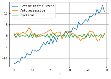
Figure 1: Three Time Series
Figure 1 illustrates three different time series models. The deterministic trend model exhibit random disturbances around a linear upward trend determined by the constants \(\beta_0\) and \(\beta_1\). The first order autoregressive time series model is one that depends on its past value, leading to persistence (random) fluctuations around zero. The cyclical model has periodic (deterministic) fluctuations around zero.
Characterizing Time Series (up to a point)
Characterizing a time series is a challenging task, as it involves describing an entire family of random variables. To make this more tractable, we often focus on the first two moments: the mean and the variance (or the covariance structure). Moments play a key role in describing the properties of random variables, and the first two are particularly significant. In the case of normally distributed random variables, these two moments completely define the distribution, making them especially useful in time series analysis.
To start, let’s define the mean of our time series. We’ll denote it by \(\mu_t = E[Y_t]\), which captures the expected value of the random variable at each time \(t\). Beyond the mean, random variables typically have covariance, but in the context of time series, we’re particularly interested in how this covariance behaves over time. This brings us to the concept of the autocovariance function, which measures the relationship between the values of a time series at different time points. For a time series \(\{Y_t\}\) the autocovariance function is defined as: \[ \gamma_t(\tau) = \mathbb E\left[ (Y_t - \mathbb EY_t) (Y_{t+\tau} - \mathbb EY_{t+\tau})’\right] \] where \(\tau\) is the time lag and the subscript \(t\) highlights that the autocovariance may depend on the specific time point.
Let the time series \(Y_t\) be defined as: \[ Y_t = \sqrt{t} \cdot \epsilon_t + \alpha \sqrt{t} \cdot \epsilon_{t-1}, \] where \(\epsilon_t \sim \mathcal{N}(0, \sigma^2)\) are independent, identically distributed noise terms and \(\alpha\in\mathbb R\).
The mean of this time series is given by \(\mu_t = 0\) for all \(t\). The autocovariance function is given by: \[ \gamma_t(\tau) = \begin{cases} t \sigma^2 (1 + \alpha^2), & \text{if } \tau = 0, \\ \alpha \sigma^2 \sqrt{t(t+1)}, & \text{if } |\tau| = 1, \\ 0, & \text{if } |\tau| > 1. \end{cases}. \]
If the autocovariance function \(\gamma_t(\tau)\) depends on both \(t\) and \(\tau\), as in Example , then the time series exhibits temporal heterogeneity. The relationship between \(Y_t\) and \(Y_{t+\tau}\) is determined not only by \(\tau\), the “distance” between the elements in the series, but by the absolute index. In the example, if \(t’ > t\), then \(|\gamma_{t’}(1)| > |\gamma_{t}(1)|\), that is, the magnitude of the first order autocovariance increasing in time \(t\). A series exhibiting such behavior is said to be nonstationary.
We’ll begin our analysis by considering only time series that do not exhibit this kind of behavior.
A time series is covariance stationary if
- \(E\left[Y_t^2\right] = \sigma^2 < \infty\) for all \(t\in T\).
- \(E\left[Y_t\right]=\mu\) for all \(t\in T\).
- \(\gamma_t(\tau) = \gamma(\tau)\) for all \(t,t+\tau \in T\).
Covariance stationary processes have an element of “sameness” because some of their key statistical properties do not change over time. This consistency makes them important for both theoretical and practical reasons: they simplify modeling and forecasting, provide tractable analytical results, and allow the use of powerful statistical tools. Many economic and financial models require covariance stationarity to ensure meaningful and interpretable relationships between variables.
We can say a bit more about the autocovariance function. First, the autocovariance function is symmetric in the sense that \(\gamma(\tau) = \gamma(-\tau)\). Second the \(\tau\)th autocovariance is bounded by the covariance (or 0th order autocovariance) \(\gamma_t(0)\). To see this, use the Cauchy-Schwarz inequality:
\begin{multline} \bigl|\gamma(\tau)\bigr| = \Bigl|\mathbb{E}\bigl[(Y_t - \mathbb{E}[Y_t]) (Y_{t+\tau} - \mathbb{E}[Y_{t+\tau}])’\bigr]\Bigr| \;\le\; \sqrt{\mathbb{E}\bigl[|Y_t - \mathbb{E}[Y_t]|^2\bigr] \,\mathbb{E}\bigl[|Y_{t+\tau} - \mathbb{E}[Y_{t+\tau}]|^2\bigr]} \\ = \sqrt{\gamma(0)\gamma(0)} = \gamma(0). \end{multline}
Thus in a covariance‐stationary process, the autocovariance function “behaves like a normal covariance” in the sense that it depends only on the lag and shares many of the same properties you would expect from a static covariance structure. In particular, we can define the autocorrelation function:
\begin{align} \rho(\tau) = \frac{\gamma(\tau)}{\gamma(0)}. \end{align}
We know \(\left|\rho(\tau)\right| \le 1\) for all \(\tau\), just like a regular covariance. Finally, a word about language: covariance-stationarity is sometimes referred to as “weak stationarity” because this concept only involves the invariance of the first two moments of the series. Confusingly, this is also sometimes just referred to as “stationarity.” We’ll talk about another notion of stationarity towards the end of the lecture.
Building covariance stationary processes. Covariance stationarity is an appealing property for a time series. We’ll focus on the construction of such processes, starting from one of the simplest covariance staitonary processes, called white noise. We’ll then build more general covariance stationary processes by taking linear combinations of white noise. Later we’ll show that this set of linear processes can mimic any covariance stationary process using the Wold Representation.
A covariance stationary process \(\{Z_t\}\) is called white noise if it satisfiess
- \(\mathbb E[Z_t] = 0\).
- \(\gamma(0) = \sigma^2\).
- \(\gamma(\tau) = 0\) for \(\tau \ne 0\).
This process is sometimes written as \(Z_t\sim WN(0,\sigma^2)\). They are kind of boring on their own, but using them we can construct arbitrary stationary processes. A special case is given by \(Z_t \stackrel{i.i.d.}{\sim}N(0,\sigma^2)\).
ARMA Processes
We’ll first start with a finite-order moving average process. This process is simply a (finite) linear combination of white noise random variables:
Let \(Z_t \sim WN(0,\sigma^2)\) and let \(\theta_j \in \mathbb R\) for \(j = 1,\ldots,q\). The moving order process of order \(q\), or MA(\(q\)), is given by:
\begin{align} Y_t = Z_t + \theta_1 Z_{t-1} + \ldots + \theta_q Z_{t-q}. \end{align}
Before proceeding with the analysis of the MA(\(q\)) model, we’ll introduce some important tools: the lag operator and lag polynomial. The lag operator \( L \) is a fundamental concept in time series analysis. For any time series \( Y_t \), the lag operator is defined as: \[ L Y_t = Y_{t-1}. \] Applying the lag operator \( k \) times corresponds to \(L^k Y_t = Y_{t-k}\). Informally, think of \( L \) as a “backward shift” in time. The lag operator provides a compact way to express time series processes like MA(\( q \)). A lag polynomial extends the idea of the lag operator by forming polynomials in \( L \). For example, consider a polynomial \( \Theta(L) \) of degree \( q \): \[ \theta(L) = 1 + \theta_1 L + \theta_2 L^2 + \ldots + \theta_q L^q. \] The MA(\( q \)) process can now be expressed succinctly as: \[ y_t = \theta(L) \epsilon_t, \] where \( \theta(L) \) is applied to \( \epsilon_t \) to generate \( y_t \). For our purposes, lag polynomials behave similarly to regular polynomials in algebra. Operations like addition, subtraction, multiplication, and factorization apply in much the same way. For example:\( \theta_1(L) + \theta_2(L) \) combines terms as usual and \( \theta_1(L) \theta_2(L) \) expands like a product of ordinary polynomials.
Now we’ll show that the MA(\(q\)) is always covariance stationary. Consider first the mean \[ \mathbb E[Y_t] = \mathbb E[Z_t] + \theta_1 \mathbb E[Z_{t-1}] + \ldots + \theta_q \mathbb E[ Z_{t-q}] = 0. \] This clearly does not depend on time. Next, consider the autocovariance, there are three cases:
Case \(\tau = 0\): The autocovariance at lag 0, \(\gamma(0)\), is simply the variance of \(Y_t\): \[ \gamma(0) = \text{Var}(Y_t) = \text{Var}\left(Z_t + \theta_1 Z_{t-1} + \ldots + \theta_q Z_{t-q}\right). \] Since the \(Z_t\) terms are white noise: \[ \gamma(0) = \sigma^2 \left(1 + \theta_1^2 + \ldots + \theta_q^2\right). \]
Case \(0 < \tau \leq q\): For \(0 < \tau \leq q\), the autocovariance at lag \(\tau\) is: \[ \gamma(\tau) = \mathbb{E}\left[(Y_t - \mathbb{E}[Y_t])(Y_{t+\tau} - \mathbb{E}[Y_{t+\tau}])\right] = \mathbb{E}\left[Z_t (\theta_\tau Z_{t-\tau})\right]. \]
Case \(\tau > q\): For lags beyond \(q\): \[ \gamma(\tau) = 0, \quad \text{since there is no overlap of terms.} \]
In sum, \[γ(τ) =
\begin{cases} \sigma^2 (\theta_\tau + \theta_1 \theta_{\tau-1} + \ldots + \theta_q \theta_{\tau-q}), & 0 < \tau \le q, \\ 0, & \tau > q. \end{cases}
\] The autocovariances depend solely on the lag \(\tau\). So the process is covariance stationary. The autocovariance is zero beyond \(q\) lags.
The processes \(\{Y_t\}\) is said to be an ARMA(\(p,q\)/) process if \(\{Y_t\}\) is stationary and if it can be represented by the linear difference equation: \[ Y_t = \phi_1 Y_{t-1} + \ldots \phi_p Y_{t-p} + Z_t + \theta_1 Z_{t-1} + \ldots + \theta_q Z_{t-q} \] with \(\{Z_t\} \sim WN(0,\sigma^2)\). Using the lag operator \(LX_t = X_{t-1}\) we can write: \[ \phi(L)Y_t = \theta(L)Z_t \] where \[ \phi(z) = 1 - \phi_1 z - \ldots \phi_p z^p \mbox{ and } \theta(z) = 1 + \theta_1 z + \ldots + \theta_q z^q. \] Special cases:
- \(AR(1) : Y_t = \phi_1 Y_{t-1} + Z_t\).
- \(MA(1) : Y_t = Z_t + \theta_1 Z_{t-1}\).
- \(AR(p)\), \(MA(q)\), \(\ldots\)
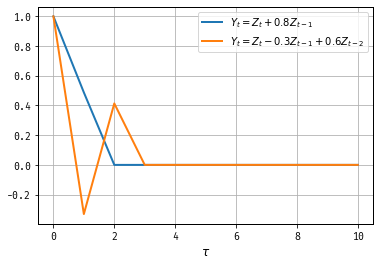
Figure 2: Autocovariance Functions of Two MA Processes
talk about these two ACFs
The plotted Autocovariance Functions (ACF) for the two Moving Average (MA) processes demonstrate key characteristics of MA models, particularly in their decay patterns:
\(Y_t = Z_t + 0.8Z_{t-1}\): This is an MA(1) process. The ACF exhibits a spike at \(\tau = 1\), and zero autocovariances for lags greater than one. This is typical for MA(1) processes, where the correlation exists only between adjacent terms and disappears entirely beyond the first lag.
\(Y_t = Z_t - 0.3Z_{t-1} + 0.6Z_{t-2}\): This is an MA(2) process. The ACF shows non-zero values at \(\tau = 1\) and \(\tau = 2\), reflecting the two-period dependency introduced by the lag terms. Beyond lag 2, the autocovariance becomes zero, as there is no third-period memory or influence.
The plots highlight that MA(q) processes have autocovariance functions with non-zero values up to the q-th lag, after which they drop to zero. This sharp cutoff is a defining feature of moving average processes, contrasting with the slow decay often observed in autoregressive (AR) processes.
AR(1)
Let’s return to Example , substituting the normal disturbances for more general white noise: \[ Y_t = \phi_1 Y_{t-1} + Z_t. \] This can be viewed as a linear difference equation, and so we can solve backwards for \(y_t\) as a function \(z_t\) via backwards substitution:
\begin{eqnarray} Y_t &=& \phi_1(\phi_1 Y_{t-2} + Z_{t-1}) + Z_{t}\\ &=& Z_t + \phi_1 Z_{t-1} + \phi_1^2 Z_{t-2} +\ldots \\ &=& \sum_{j=0}^{\infty} \phi_1^j Z_{t-j}. \end{eqnarray}
How do we know whether this is a covariance stationary process? Things are a little bit trickier than the MA case we have already studied: the AR(1) is a function of infinitely many \(z\)s. To determine whether this AR(1) process is covariance stationary, we need to examine if \( y_t \) converges to a random variable given the infinite history of innovations. This requires introducing the concept of mean square convergence.
A sequence of random variables \(\{Y_t\}\) is said to converge in mean square to a random variable \(Y\) if the expectation of the squared differences between them approaches zero as \(t\) tends to infinity. Formally, this is expressed as: \[ \mathbb{E}\left[(Y_t - Y)^2\right] \rightarrow 0 \quad \text{as} \quad t \rightarrow \infty. \] The idea of mean square convergence is closely related to the convergence of infinite series in the deterministic setting, such as \(\sum_{j=0}^\infty a_j\). To ensure the AR(1) process converges, and thus can be considered covariance stationary, we verify that the infinite sum of the coefficients \(\phi_1^j\) multiplied by the white noise terms \(z_{t-j}\) does not diverge.
AR(2)
Consider now the AR(2) model: \[ Y_t = \phi_1 Y_{t-1} + \phi_2 Y_{t-2} + Z_t \] Which means \[ \phi(L) Y_t = Z_t, \quad \phi(z) = 1 - \phi_1 z - \phi_2 z^2 \] Under what conditions can we invert \(\phi(\cdot)\)? Factoring the polynomial \[ 1 - \phi_1 z - \phi_2 z^2 = (1-\lambda_1 z) (1-\lambda_2 z) \] Using the above theorem, if both \(|\lambda_1|\) and \(|\lambda_2|\) are less than one in length (they can be complex!) we can apply the earlier logic succesively to obtain conditions for covariance stationarity.
Note: \(\lambda_1\lambda_2 = -\phi_2\) and \(\lambda_1 + \lambda_2 = \phi_1\)
\begin{eqnarray}\left[\begin{array}{c}Y_t \\ Y_{t-1} \end{array}\right] = \left[\begin{array}{cc}\phi_1 & \phi_2 \\ 1 & 0 \end{array}\right] \left[\begin{array}{c}Y_{t-1} \\ Y_{t-2} \end{array}\right] + \left[\begin{array}{c}\epsilon_t\\ 0 \end{array}\right]\end{eqnarray}
\({\mathbf Y}_t = F {\mathbf Y}_{t-1} + {\mathbf \epsilon_t}\)
\(F\) has eigenvalues \(\lambda\) which solve \(\lambda^2 - \phi_1 \lambda - \phi_2 = 0\) Multiplying and using the symmetry of the autocovariance function:
\begin{eqnarray} Y_t &:&\gamma(0) = \phi_1\gamma(1) + \phi_2\gamma(2) + \sigma^2 \\ Y_{t-1} &:& \gamma(1) = \phi_1\gamma(0) + \phi_2\gamma(1) \\ Y_{t-2} &:& \gamma(2) = \phi_1\gamma(1) + \phi_2\gamma(0) \\ &\vdots& \\ Y_{t-h} &:& \gamma(h) = \phi_1\gamma(h-1) + \phi_2\gamma(h-2) \end{eqnarray}
We can solve for \(\gamma(0), \gamma(1), \gamma(2)\) using the first three equations: \[ \gamma(0) = \frac{(1-\phi_2)\sigma^2}{(1+\phi_2)[(1-\phi_2)^2 - \phi_1^2]} \] We can solve for the rest using the recursions.
Note pth order AR(1) have autocovariances / autocorrelations that follow the same pth order difference equations.
Autocorrelations: call these Yule-Walker equations following the work of Yule (1927) and Walker (1931).
Large Samples Revisited
We’ll show a weak law of large numbers and central limit theorem applies to this process using the Beveridge and Nelson (1981) decomposition following Phillips and Ploberger (1996). For the MA(\(q\)), setting \(q_0 = 1\) (a normalization), we can write \(\theta(\cdot)\) in a Taylor expansion-ish sort of way:
\begin{eqnarray} \theta(L) &=& \sum_{j=0}^q \theta_j L^j, = \left(\sum_{j=0}^q \theta_j - \sum_{j=1}^q \theta_j\right) + \left(\sum_{j=1}^q \theta_j - \sum_{j=2}^q \theta_j\right)L \nonumber \\ &~&+ \left(\sum_{j=2}^q \theta_j - \sum_{j=3}^q \theta_j\right)L^2 + \ldots \nonumber \\ &=& \sum_{j=0}^q \theta_j + \left(\sum_{j=1}^q\theta_j\right)(L-1) + \left(\sum_{j=2}^q\theta_j\right)(L^2-L) + \ldots\nonumber\\ &=& \theta(1) + \widehat\theta_1(L-1) + \widehat\theta_2 L (L-1) + \ldots \nonumber\\ &=& \theta(1) + \widehat\theta(L)(L-1) \nonumber \end{eqnarray}
Here \(\widehat{\theta}_i = \sum_{j=i}^q \theta_j\). Thus, we can write \(y_t\) as \[ y_t = \theta(1) \epsilon_t + \hat\theta(L)\epsilon_{t-1} - \hat\theta(L)\epsilon_{t} \] An average of \(y_t\) cancels most of the second and third term … \[ \frac1T \sum_{t=1}^T y_t = \frac{1}{T}\theta(1) \sum_{t=1}^T \epsilon_t + \frac1T\left(\hat\theta(L)\epsilon_0 - \hat\theta(L)\epsilon_T\right) \] We have \[ \frac{1}{\sqrt{T}}\left(\hat\theta(L)\epsilon_0 - \hat\theta(L)\epsilon_T\right) \rightarrow 0. \] Then we can apply the WLLN / CLT for iid sequences (from the beginning of the lecture) with Slutzky’s Theorem to deduce that \[ \frac1T \sum_{t=1}^T y_t \rightarrow 0 \mbox{ and } \frac{1}{\sqrt{T}}\sum_{t=1}^T y_t \rightarrow N(0, \sigma^2 \theta(1)^2). \]
A time series is strictly stationary if for all \(t_1,\ldots,t_k, k, h \in T\) if \[ Y_{t_1}, \ldots, Y_{t_k} \sim Y_{t_1+h}, \ldots, Y_{t_k+h} \]
We started this lecture with a refresher on the WLLN and CLT for sums of independent random variables. As emphasized, time series data, however, are often not independent, which necessitates the use of more advanced tools to analyze them effectively. And covariance staionarity is in general not enough. We instead rely on /ergodicity/—a property that helps us understand under what conditions time averages (i.e., averages calculated over time) converge to population averages (i.e., expected values). This property is important make inferential statements about the entire process based on a single, sufficiently long observation path. Essentially, for ergodic processes, “time averages are equivalent to space averages.”
A stationary process is classified as ergodic if, for any two bounded and measurable functions \( f: \mathbb R^k \rightarrow \mathbb R \) and \( g: \mathbb R^l \rightarrow \mathbb R \), the following condition holds: \[ \lim_{n \rightarrow \infty} \left|\mathbb{E} \left[ f(y_t,\ldots,y_{t+k})g(y_{t+n},\ldots,y_{t+n+l})\right]\right| - \left|\mathbb{E} \left[ f(y_t,\ldots,y_{t+k})\right]\right|\left|\mathbb{E}\left[g(y_{t+n},\ldots,y_{t+n+l})\right]\right| = 0 \]
At an intuitive level, a process is ergodic if the dependency between an event today and an event at some future horizon diminishes as the time horizon increases. An important result involving ergodic processes is the Ergodic Theorem. If \( \{y_t\} \) is a strictly stationary and ergodic process, and \( \mathbb E[y_1] < \infty \), then the time average of the process converges to the population average: \[ \frac{1}{T} \sum_{t=1}^{T} y_t \longrightarrow \mathbb{E}[y_1] \] This theorem assures us that time averages are consistent estimators of the population mean for ergodic processes. The Central Limit Theorem for strictly stationary and ergodic processes provides us with distributional results. If \( \{y_t\} \) is such a process with \( \mathbb{E}[y_1] < \infty \), \( \mathbb{E}[y_1^2] < \infty \), and \( \bar\sigma^2 = \text{Var}(T^{-1/2} \sum y_t) \rightarrow \bar\sigma^2 < \infty \), then: \[ \frac{1}{\sqrt{T} \bar\sigma_T} \sum_{t=1}^{T} y_t \rightarrow N(0,1) \] Here are some facts about ergodicity:
- IID Sequences: Independent and identically distributed (IID) sequences are both stationary and ergodic naturally.
- Functions of Ergodic Processes: If \( \{Y_t\} \) is strictly stationary and ergodic, and \( f: \mathbb R^\infty \rightarrow \mathbb R \) is measurable, then the sequence \( Z_t = f(\{Y_t\}) \) is also strictly stationary and ergodic.
Consider an \( MA(\infty) \) process with iid Gaussian white noise: \[ Y_t = \sum_{j=0}^{\infty} \theta_j \epsilon_{t-j}, \quad \sum_{j=0}^{\infty} |\theta_j| < \infty \] For this process, \( \{Y_t\}, \{Y_t^2\}, \text{ and } \{Y_tY_{t-h}\} \) are ergodic. This implies: \[ \frac{1}{T} \sum_{t=0}^{\infty} Y_t \rightarrow \mathbb{E}[Y_0], \quad \frac{1}{T} \sum_{t=0}^{\infty} Y_t^2 \rightarrow \mathbb{E}[Y_0^2], \quad \frac{1}{T} \sum_{t=0}^{\infty} Y_t Y_{t-h} \rightarrow \mathbb{E}[Y_0 Y_{-h}] \] A sequence \( \{Z_t\} \) is termed a Martingale Difference Sequence (MDS) with respect to information sets \( \{\mathcal{F}_t\} \) if: \[ E[Z_t | \mathcal{F}_{t-1}] = 0 \quad \text{for all} \; t \] For a martingale difference sequence \( \{Y_t, \mathcal{F}_t\} \) satisfying \( E[|Y_t|^{2r}] < \Delta < \infty \) for some \( r > 1 \), and all \( t \):
- The sample average \( \bar{Y}_T = T^{-1} \sum_{t=1}^T Y_t \stackrel{p}{\longrightarrow} 0 \).
- If \( \text{Var}(\sqrt{T} \bar{Y}_T) = \bar{\sigma}_T^2 \rightarrow \sigma^2 > 0 \), then:
\[ \sqrt{T} \bar{Y}_T / \bar{\sigma}_T \Longrightarrow \mathcal{N}(0,1) \]
Consider an investor making decisions between a stock with real return \( r_t \) and a nominal bond with guaranteed return \( R_{t-1} \) subject to inflation risk \( \pi_t \). Assuming risk neutrality and no arbitrage implies: \[ \mathbb{E}_{t-1}[r_t] = \mathbb{E}_{t-1}[R_{t-1} - \pi_t] \] This can be rewritten as: \[ 0 = r_t + \pi_t - R_{t-1} - \underbrace{\left((r_t - \mathbb{E}_{t-1}[r_t]) + (\pi_t - \mathbb{E}_{t-1}[\pi_t])\right)}_{\eta_t} \] Here, \( \eta_t \) is an expectation error and, under rational expectations, \( \mathbb{E}_{t-1}[\eta_t] = 0 \). Therefore, \( \eta_t \) forms a Martingale Difference Sequence, a fact we will explore further in Generalized Method of Moments (GMM) estimation later in the course.
The Trinity In Macro
Empirical Time Series: Log Real GDP, PCE Inflation, and Federal Funds Rate
Time series analysis is widely applied in macroeconomics to understand and forecast key economic indicators. In this subsection, we’ll briefly discuss three such empirical time series: the logarithm of real Gross Domestic Product (GDP), Personal Consumption Expenditures (PCE) inflation, and the federal funds rate.
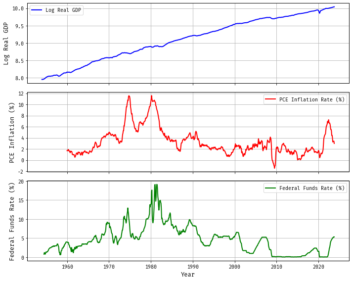
Figure 3: Three Macroeconomic Time Series