Trends in Time Series
Lecture Objective: Understand the basic of deterministic and stochastic trends. Give a heuristic introduction to large sample theory. Additional Readings: You can find background in Hamilton (1994) chapters 15-16 and Davidson and MacKinnon (2003). We’ll discuss the results in Nelson and Plosser (1982) in some detail in the lecture.
A common method for analyzing macroeconomic time series is to decompose them into two distinct components: trend and cycle. This approach allows economists to better understand the underlying causes and effects of economic phenomenon at two different frequencies.
To illustrate, consider the example of real per capita GDP, denoted as \( gdp_t \), which represents the economic output per individual in the United States. In this decomposition framework, we express the natural logarithm of per capita GDP, \( y_t \), as the sum of its trend component and its fluctuations. Mathematically, this can be represented as: \[ y_t = \ln gdp_t = trend_t + fluctuations_t \] In this equation, \( trend_t \) might represent the “underlying” growth trajectory of the economy, while \( fluctuations_t \) are short-term variations around this trend, known as cyclical movements.
Separating trend from cycle is a difficult problem. Take the case of log GDP: while the total data is compiled by the Bureau of Economic Analysis, the trend and cycle are not observed. In general, we’ll need additional assumptions to identify these two components of a given time series. In this lecture we’ll talk about deterministic and stochastic trends.
Deterministic Trends
For much of the 20th century, economists thought the underlying economic growth was largely predictable with temporary business cycles. An example of this way of thinking was the large scale econometric model of Tinbergen (1939), vol. 1.
We’ll focus the linear deterministic trend model. Consider the model:
\begin{align} y_t = \beta_1 + \beta_2 t + u_t. \end{align}
Let’s make some assumptions on \(u_t\): \[ \mathbb E[u_t] = 0 \text{ and } \mathbb V[u_t^2] = \sigma^2. \] Let’s further assume that \(u_t\) is covariance stationary process. This kind of model has a few interesting implications. Under our assumptions on \(u_t\), the future value \( y_{t+h} \), for a large horizon \( h \), can be predicted by extending the trend component: \[ \mathbb E_t[y_{t+h}] \approx \beta_1 + \beta_2 (t+h) \text{ as \(h\) becomes large}. \] Thus, the long-run forecast of \( y_t \) becomes increasingly determined by the trend, and as \( u_t \) converges to its unconditional expectation. As \( h \) becomes large, the prediction error variance for \( y_{t+h} \) is bounded (it’s simply \(\sigma^2\).)
To implement this trend-cycle decomposition, we can estimate Equation . After estimating \(\beta_1\) and \(\beta_2\), we can obtain a decomposition:
\begin{eqnarray} y_t &=& \widehat{trend}_t + \widehat{fluctuations}_t \nonumber \\ &=& (\hat{\beta}_1 + \hat{\beta}_2 t) + ( y_t - \hat{\beta}_1 - \hat{\beta}_2t). \end{eqnarray}
When \(y_t\) is a logged variable, the coefficient \(\beta_2\) has the interpretation of an average growth rate. Figure 1 shows the trend and fluctuations for United States annual log GNP from 1909-1970. The data come from Nelson and Plosser (1982) and the coefficients are estimated using ordinary least squares.
The estimated coefficient \(\hat{\beta}_2\) is 0.031. This gives an average annual growth rate of about 3.1% over the period from 1909 to 1970. This indicates that, despite the fluctuations typical of economic activity, the underlying long-term trend was one of moderate growth. The Great Depression is clearly visible in the cycle.
[0;31m---------------------------------------------------------------------------[0m
[0;31mNameError[0m Traceback (most recent call last)
[0;32m<ipython-input-1-bf73901e5db8>[0m in [0;36m<module>[0;34m[0m
[1;32m 20[0m [0;31m# Assign the inferred column names[0m[0;34m[0m[0;34m[0m[0;34m[0m[0m
[1;32m 21[0m [0mdata[0m[0;34m.[0m[0mcolumns[0m [0;34m=[0m [0mcolumn_names[0m[0;34m[0m[0;34m[0m[0m
[0;32m---> 22[0;31m [0mdata[0m[0;34m[[0m[0;34m'Year'[0m[0;34m][0m [0;34m=[0m [0mp[0m[0;34m.[0m[0mto_datetime[0m[0;34m([0m[0mdata[0m[0;34m[[0m[0;34m'Year'[0m[0;34m][0m[0;34m,[0m [0mformat[0m[0;34m=[0m[0;34m'%Y'[0m[0;34m)[0m[0;34m[0m[0;34m[0m[0m
[0m[1;32m 23[0m [0mdata[0m [0;34m=[0m [0mdata[0m[0;34m.[0m[0mreplace[0m[0;34m([0m[0;36m0[0m[0;34m,[0m [0mnp[0m[0;34m.[0m[0mnan[0m[0;34m)[0m[0;34m.[0m[0mset_index[0m[0;34m([0m[0;34m'Year'[0m[0;34m)[0m[0;34m.[0m[0mto_period[0m[0;34m([0m[0;34m'A'[0m[0;34m)[0m[0;34m[0m[0;34m[0m[0m
[1;32m 24[0m [0;32mfor[0m [0mc[0m [0;32min[0m [0mdata[0m[0;34m.[0m[0mcolumns[0m[0;34m:[0m[0;34m[0m[0;34m[0m[0m
[0;31mNameError[0m: name 'p' is not defined
Econometrics of Deterministic Trend Models. You’ve surely gone through the analysis of this regression model for cross sectional data. Things are a bit different for the deterministic trend model. In fact, there are several difficulties associated with large sample analysis of the estimators \(\hat{\beta}_{1,T}\) and \(\hat{\beta}_{2,T}\). Taking \(x_t = \left[1, t\right]’\),
- The matrix \(\frac{1}{T} \sum x_t x_t’\) does not converge to a non-singular matrix \(Q\) as the time trend grows without bound.
- In a time series model, the disturbances \(u_t\) are in general dependent. This will change the limiting distribution of quantities such as \(\sqrt{T} \frac{1}{T} \sum x_t u_t\).
- If the \(u_t\)’s are serially correlated, then the OLS estimator will in general be inefficient. More sophisticated estimation techniques, like Generalized Least Squares (GLS), might be necessary to achieve efficiency.
Roughly speaking, convergence rates tell us how fast we can learn the``true’’ value of a parameter in a sampling experiment. In “standard” OLS then the variance of the \(\hat\beta\) converges to zero at rate \(1/T\). This isn’t true for models with deterministic trends. Let’s look at the distributions of \(\sqrt{T}(\hat\beta_0 - \beta_0)\) and \(\sqrt{T}(\hat\beta_1 - \beta_1)\).
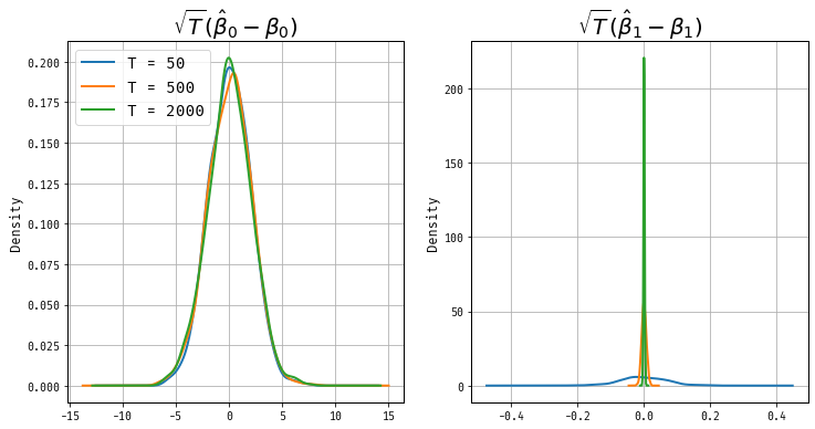
Figure 1: Sampling Distribution of (widehatbeta)
Figure 1 displays the sampling distributions for \(\widehat \beta_0\) and \(\widehat \beta_1\). The standardized estimate of \(\widehat\beta_0\) is stabilized at normal dstirbution. However the estimate \(\sqrt{T}(\widehat\beta_1 - \beta_1)\) is clearly degenerating to a point mass at zero as \(T\) becomes large, as its variance is shrinnking rapidly. We’ll analysis this asymptotic result now.
We’ll begin with some algebraic identities that will be helpful.
\begin{eqnarray*} \sum_{t=1}^T 1 = T,\quad \sum_{t=1}^T t = \frac{T(T+1)}{2}, \text{ and } \sum_{t=1}^T t^2 = \frac{T(T+1)(2T+1)}{6}. \end{eqnarray*}
Using these identitites, it’s easy to see that the matrix \[ \frac{1}{T} \sum x_t x_t’ = \frac{1}{T} \left( \begin{array}{cc} \sum 1 & \sum t \\ \sum t & \sum t^2 \end{array} \right) \] does not converge at \(T\) becomes large. On the the hand \[ \frac{1}{T^{\textcolor{red}{3}}} \sum x_t x_t’ \longrightarrow \left( \begin{array}{cc} 0 & 0 \\ 0 & 1/3 \end{array} \right) \] is singular and not invertible! Thus, deterministic trends change the rate of convergence of estimators. It turns out that \(\hat{\beta}_{1,T}\) and \(\hat{\beta}_{2,T}\) have different asymptotic rates of convergence. In particular, we will learn faster about the slope of the trend line than the intercept.
To analyze the asymptotic behavior of the estimators we define the matrix \[ G_T = \left( \begin{array}{cc} 1 & 0 \\ 0 & T \end{array} \right). \] Note that the matrix is equivalent to its transpose, that is, \(G_T = G_T’\). We will analyze the following quantity \[ G_T(\hat{\beta}_T - \beta) = \left( \frac{1}{T} \sum G_T^{-1} x_t x_t’G_T^{-1} \right)^{-1} \left( \frac{1}{T}\sum G_T^{-1} x_t u_t \right). \] It can be easily verified that \[ \frac{1}{T} \sum G_T^{-1} x_t x_t’ G_T^{-1} = \frac{1}{T} \left( \begin{array}{cc} \sum 1 & \sum t/T \\ \sum t/T & \sum (t/T)^2 \end{array} \right) \longrightarrow Q, = \left( \begin{array}{cc} 1 & 1/2 \\ 1/2 & 1/3 \end{array} \right). \] The term \(\frac{1}{T} \sum G_T^{-1} x_t u_t\) has the components \(\frac{1}{T} \sum u_t\) and \(\frac{1}{T} \sum (t/T) u_t\) which converge in probability to zero based on the weak law of large numbers for non-identically distributed random variables. Note that without the proper standardization \(\frac{1}{T} \sum t u_t\) will not converge to its expected value of zero. The variance of the random variable \(T u_T\) is getting larger and larger with sample size which prohibits the convergence of the sample mean to its expectation.
With this, we can describe some asymptotic results: \[ y_t = \beta_1 + \beta_2 t + u_t, \quad u_t \stackrel{i.i.d.}{\sim} (0,\sigma^2). \] Let \(\hat{\beta}_{i,T}\), \(i=1,2\) be the OLS estimators of the intercept and slope coefficient, respectively. Then
\begin{eqnarray} \hat{\beta}_{1,T} -\beta_1 & \stackrel{p}{\longrightarrow} & 0 \label{eq_rint}\\ T(\hat{\beta}_{2,T} - \beta_2) & \stackrel{p}{\longrightarrow} & 0 \label{eq_rslp}. \end{eqnarray}
For the sampling distribution, consider the quantity \[ \sqrt{T} G_T (\hat{\beta}_T - \beta) = \left[ \begin{array}{c} \sqrt{T}(\hat{\beta}_{1,T} - \beta) \\ T^{3/2}(\hat{\beta}_{2,T} - \beta_2) \end{array} \right]. \] This is equal to \[ \left( \frac{1}{T} \sum G_T^{-1} x_t x_t’ G_T^{-1} \right)^{-1} \left( \frac{1}{\sqrt{T}}\sum G_T^{-1} x_t u_t \right). \] In this setup, the matrix \(\frac{1n}{T} \sum G_T^{-1} x_t x_t’ G_T^{-1}\) converges to a non-singular matrix \(Q\) as discussed earlier. Consider now: \[ \left( \frac{1}{\sqrt{T}}\sum G_T^{-1} x_t u_t \right) = \left[ \begin{array}{c} \frac{1}{\sqrt{T}} \sum u_t \\ \frac{1}{\sqrt{T}} \sum \left(\frac{t}{T}\right) u_t \end{array} \right]. \] The second term is in this is an indepedendent but not identically distributed random variable because the scaling \( \left(\frac{t}{T}\right) \) changes over time. We can invoke a central limit theorem for these kinds of random variables due to Lyapunov–see Casella and Berger (2002) Theorem 27.3.1. We deduce that both elements of the vector have a limiting normal distribution. Next, we can use Cramer-Wold theorem—for details see Casella and Berger (2002), Theorem 5.5.3—to conclude that a linear combination of these elements will also have a limiting normal distribution, allowing us to analyze the behavior of the full vector. Taken together, the sampling distribution of the OLS estimators has the following large sample behavior \[ \sqrt{T} G_T (\hat{\beta}_T - \beta) \Longrightarrow {\cal N}(0,\sigma^2Q^{-1}). \] Having said all this. When we consider the case where the variance is unknown: \[ \hat \sigma^2 = \frac{1}{T-2}\sum(y_t - \hat\beta_1 - \hat\beta_2 t)^2, \] under standard conditions, \(\hat{\sigma}^2\) will consistently estimate \(\sigma^2\), and the asymptotic normality results still hold, meaning that the scaled estimators, adjusted for unknown variance, converge to a normal distribution with the true variance replaced by \(\hat{\sigma}^2\). espite the fact that \(\beta_1\) and \(\beta_2\) have different asymptotic rates of convergence, the t statistics still have \(N(0,1)\) limited distribution because the standard error estimates have offsetting behaviour.
OLS and Serial Dependence
Let’s ignore the constant term and consider the simplified regression
\begin{align} y_t = \beta t + u_t. \end{align}
In times series models, it’s likely that the \(u_t\) are serially correlated, that is, \(\mathbb E[u_{t}u_{t-h}] \not= 0\) for some \(h\). This means that OLS will be inefficient. That is, the OLS estimator will not achieve the smallest possible variance among unbiased estimators. Let’s look at example with \(MA(1)\) errors. \[ u_t = \epsilon_t + \theta \epsilon_{t-1}, \quad \epsilon_{t} \sim iid(0,\sigma^2_\epsilon). \] It’s easy to verify that:
\begin{eqnarray} \mathbb E[u_t^2] & = & \mathbb E[(\epsilon_t + \theta \epsilon_{t-1})^2] = (1+\theta^2)\sigma^2_\epsilon \\ \mathbb E[u_tu_{t-1}] & = & \mathbb E[ (\epsilon_t + \theta \epsilon_{t-1})(\epsilon_{t-1} + \theta \epsilon_{t-2})] = \theta \sigma^2_\epsilon \\ \mathbb E[u_tu_{t-h}] & = & 0 \quad h > 1. \end{eqnarray}
For the regression model , the OLS estimator is given by \[ \hat{\beta}_T - \beta = \frac{\sum tu_t}{\sum t^2}. \] To find the limiting distribution, note that \[ \frac{1}{T^3} \sum_{t=1}^T t^2 = \frac{T(T+1)(2T+1)}{6T} \longrightarrow \frac{1}{3}. \]
\begin{eqnarray} \sum t u_t & = & \sum t(\epsilon_t + \theta \epsilon_{t-1}) \nonumber \\ & = & \begin{array}{ccccc} 0 & +\epsilon_1 & +2\epsilon_2 & + 3\epsilon_3 & + \ldots \\ +\theta \epsilon_0 & + 2 \theta \epsilon_1 & + 3 \theta \epsilon_2 & + 4 \theta \epsilon_3 & + \ldots \end{array} \nonumber \\ & = & \sum_{t=1}^{T-1} (t + \theta(t+1)) \epsilon_t \; + \theta \epsilon_0 + T \epsilon_T \nonumber \\ & = & \sum_{t=1}^{T-1} (1+\theta) t \epsilon_t + \sum_{t=1}^{T-1} \theta \epsilon_t + \theta \epsilon_0 + T \epsilon_T \nonumber \\ & = & \sum_{t=1}^T (1+\theta) t \epsilon_t \underbrace{ - \theta T \epsilon_T + \theta \sum_{t=1}^T \epsilon_{t-1} }_{\mbox{asymp. negligible}}. \end{eqnarray}
After standardization by \(T^{-3/2}\) we obtain
\begin{eqnarray*} T^{-3/2} \sum tu_t = \frac{1}{\sqrt{T}} (1+\theta) \sum_{t=1}^T (t/T) \epsilon_t - \frac{1}{\sqrt{T}} \theta \epsilon_T + \frac{\theta}{T} \frac{1}{\sqrt{T}} \sum_{t=1}^T \epsilon_{t-1}. \end{eqnarray*}
- First term obeys CLT
- Second Term goes to zero
- Third Term goes to zero
Thus , \[ T^{3/2}( \hat{\beta}_T - \beta) \Longrightarrow \big(0,3\sigma^2_\epsilon (1+\theta)^2 \big). \] Consider the following model with \(iid\) disturbances \[ y_t = \beta t + u_t, \quad u_t \sim iid(0,\sigma_\epsilon^2(1+\theta^2)). \] The unconditional variance of the disturbances is the same as in the model with moving average disturbances. It can be verified that \[ T^{3/2}( \hat{\beta}_T - \beta) \Longrightarrow \big(0,3\sigma^2_\epsilon (1+\theta^2) \big). \] If \(\theta\) is positive then the limit variance of the OLS estimator in the model with $i.i.d.$ disturbances is smaller than in the trend model with moving average disturbances. Thus, Positive serial correlated data are less informative than $i.i.d.$ data. Figure 2 displays the sampling distribution of the OLS estimator under errors with identical unconditional variance but with serial correlation (blue line) and under \(i.i.d.\) disturbances (orange dashed line). In this set of simulations, \(\beta = 0.5\), \(\theta = 0.6\), and \(\sigma_\epsilon = 1\). The sample size is given by \(T = 500\). Clearly, the estimator under serial correlation exhibits large variance, though both estimators are asymptotically unbiased.
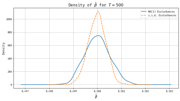
Figure 2: OLS is Inefficient Under Serially Correlated Errors
Stochastic Trends
Nelson and Plosser (1982) challenged the idea that economic activity ought to be modeled as temporary (stationary) fluctuations around a deterministic trend. They proposed that economic time series might instead be better represented by stochastic trends, where shocks have permanent effects, leading to a “random walk-like” behavior. This implies that the series does not revert to a deterministic path but can drift over time due to accumulated random changes. Such time series are known as “integrated” processes because they require differencing to achieve stationarity. Specifically, a time series that follows a stochastic trend can be modeled as an integrated process, often denoted as an \( I(1) \) process, where differencing once will result in a stationary series.
A random walk with drift follow the process \[ y_t = \phi_0 + y_{t-1} + \epsilon_t \quad \epsilon_t \sim WN(0,\sigma^2) \] The variable \(y_t\) is said to be integrated of order one.
The applied work of Nelson and Plosser (1982) came alongside important technical advances in econometrics and statistics. In an important contribution, Dickey and Fuller (1979) examined the sampling distribution of estimators for autoregressive time series with a unit root and provided tables with critical values for unit root tests. This meant researchers could formally test for the presence of unit roots in time series data, allowing for differentiation between stochastic trends and stationary fluctuations. Later Phillips (1986) and Phillips (1987) published two papers on spurious regression and time series regressions with a unit root that employ the mathematical theory of convergence of probability measures for metric spaces. This marked a ``technological breakthrough’’ and the field started to grow at an exponential rate thereafter.
Let’s return the random walk model in Example omitting drift, that is, \(\phi_0 = 0\). \[ y_t = \phi y_{t-1} + \epsilon_t, \quad \epsilon_t WN(0,\sigma^2) \] There are three cases:
- \(|\phi|<1\): stationarity! we talked about this last week
- \(|\phi|>1\): explosive! We will not analyze explosive processes in this course.
- \(|\phi|=1\). This is the unit root and will be the focus of this part of the lecture.
If \(\phi=1\) then the AR(1) model simplifies to \(y_t = y_{t-1} + \epsilon_t\) with \(\Delta=1-L\), we have \(\Delta y_t = \epsilon_t\) form a stationary process, and the random walk is integrated of order one, or \(I(1)\).
It’s important to understand the implications of a unit root process relative to those of a persist, but ultimately stationary process. For now, let’s suppose that the AR process is initialized by \(y_0 \sim {\cal N}(0,1)\). Then \(y_t\) can be expressed as \[ y_t = \phi^{t} y_0 + \sum_{\tau=1}^t \phi^{\tau -1} \epsilon_{t+1-\tau}. \] The unconditional mean of this process is given by: \[ \mathbb E[y_t] = \phi^{t-1} \mathbb E[y_0] + \sum_{\tau=1}^t \phi^{\tau -1} \mathbb E[\epsilon_\tau] = 0. \] This is true regardless of the value of \(\phi_0\). Consider now the unconditionaly variance:
\begin{eqnarray} \mathbb V[y_t] & = & \phi^{2(t-1)} \mathbb V[y_0] + \sum_{\tau=1}^t \phi^{2(\tau-1)} \mathbb V[\epsilon_\tau] \\ & = & \phi^{2(t-1)} \mathbb V[y_0] + \sigma^2 \sum_{\tau=1}^t \phi^{2(\tau-1)} \nonumber \\ & = & \left\{ \begin{array}{lclcl} \phi^{2(t-1)} \mathbb V[y_0] + \sigma^2 \frac{1 - \phi^{2t}}{1 - \phi^2} & \longrightarrow & \frac{\sigma^2}{1-\phi^2} & \mbox{if} & |\phi| < 1 \\ \mathbb V[y_0] + \sigma^2 t & \longrightarrow & \infty & \mbox{if} & |\phi| =1 \end{array} \right. \nonumber \end{eqnarray}
as \(t \rightarrow \infty\). For the random walk process, the variance grows linearly with time, ultimately leading to an infinite variance. This is in contrast to the stationary AR(1) process with \(|\phi| < 1\), where the variance approaches a constant (finite) value over time. This characteristic of a unit root process reflects the permanent effects of shocks on the series.
Consider next the conditional expectation of \(y_{t}\) given \(y_0\) is
\begin{eqnarray*} \mathbb E[y_{t}|y_0] = \phi^{\tau-1} y_0 \longrightarrow \left\{ \begin{array}{lcl} 0 & \mbox{if} & |\phi| < 1 \\ y_0 & \mbox{if} & \phi = 1 \end{array} \right\} \end{eqnarray*}
as \(t \rightarrow \infty\). In the unit root case, the best prediction of future \(y_{t}\) is the initial \(y_0\) at all horizons, that is, ``no change’’. In the stationary case, the conditional expectation converges to the unconditional mean. For this reason, stationary processes are also called ``mean reverting’’. Stationary and unit root processes differ in their behavior over long time horizons. Suppose that \(\sigma^2=1\), and \(y_0=1\). Then the conditional mean and variance of a process \(y_t\) with \(\phi = 0.995\) is given by
| Horizon \(t\) | 1 | 2 | 5 | 10 | 20 | 50 | 100 |
|---|---|---|---|---|---|---|---|
| \(\mathbb E[y_t\mid y_0]\) | 0.995 | 0.990 | 0.975 | 0.951 | 0.905 | 0.778 | 0.606 |
| \(\mathbb V[y_t \mid y_0]\) | 1.000 | 1.990 | 4.901 | 9.563 | 18.21 | 39.52 | 63.46 |
If interestered in long run predictions, very important to distinguish these two cases. But note that long run predictions face serious extrapolation problems.
Heuristic Introduction to Asymptotics of Unit Root Processes
Suppose our data is generated under the random walk of Example , and we regress \(y_t\) on a constant and a lag of itself. If we’re interest in testing the null hypothesis \(H_0: \phi = 1\), we have to find the sampling distribution of a suitable test statistic such as the \(t\) ratio \[ \frac{\hat{\phi}_T -1}{\sqrt{ \sigma^2 / \sum y_{t-1}^2 }}. \] In the last lecture, we described a variety of WLLN and CLTs for stationary processes. Unfortunately, these don’t apply in this case.
To sketch the asymptotics of the test statisticis, let’s simplify our example with \(\phi_0 = 0\), \(\sigma = 1\), and \(y_0 = 0\). Thus, the process \(y_t\) can be represented as \[ y_T = \sum_{t=1}^T \epsilon_t. \] The central limit theorem for \(i.i.d.\) random variables implies \[ \frac{y_T}{\sqrt{T} } = \frac{1}{\sqrt{T}} \sum \epsilon_t \Longrightarrow {\cal N}(0,1). \] This suggests that \[ \frac{1}{T} \sum y_t = \frac{1}{\sqrt{T}} \sum \left[ \sqrt{ \frac{t}{T} } \frac{1}{\sqrt{t}} \sum_{\tau =1}^t \epsilon_\tau \right] \] will not converge to a constant in probability but instead to a random variable. We’ll need some more probably theory to analyze this.
In our course, We used \(T = \{0, \pm 1, \pm 2, \ldots\}\). Consider instead the continous time set \(S = [0,1]\). Let’s consider random elements \(W(s)\) that correspond to functions this interval. We will place some probability \(Q\) on these functions and show that \(Q\) can be helpful in the approximation of the distribution of \(\sum y_t\) Defining probability distributions on function spaces is a pain! Let \({\cal C}\) be the space of continuous functions on the interval \([0,1]\). We will define a probability distribution for the function space \({\cal C}\). This probability distribution is called ``Wiener measure’’. Whenever we draw an element from the probability space weobtain a function \(W(s)\), \(s \in [0,1]\). Let \(Q[ \cdot ]\) denote the expectation operator under the Wiener measure.
Properties of \(W(s)\). The random function has some nice properties:
- \( W(0) = 0 \) almost surely. If we repeatedly draw functions under the Wiener measure and evaluate these functions at a particular value \(s = s’\), then \[ Q[ \{ W(s’) \le w \} ] = \frac{1}{\sqrt{2\pi s’}} \int_{-\infty}^{w} e^{- u^2/2s’} du\] that is, \[ W(s’) \sim {\cal N}(0,s’) \] If \(s’=0\) then the equations is interpreted to mean \(Q[\{W(0)=0 \}] = 1\). Thus \(W(0) = 0\) with probability one.
- \( W(s) \) has independent increments. If \[ 0 \le s_1 \le s_2 \le \ldots \le s_k \le 1 \] Then the random variables \[ W(s_2) - W(s_1), \; W(s_3) - W(s_2)\; \ldots , \; W(s_k) - W(s_{k-1}) \] are independent.
- For \(0 \leq t < s \), the increment \( W(s) - W(t) \) follows a normal distribution with mean 0 and variance \( s - t \). Note: \(W(1) \sim {\cal N}(0,1)\).
It can be shown that there indeed exists a probability distribution on \({\cal C}\) with these properties. Roughly speaking, the Wiener measure is to the theory of stochastic processes, what the normal distribution is to the theory related to real valued random variables. In the context of unit root processes and econometrics, \( W(s) \) can be thought of as the continuous-time analog of the partial sum of a random walk. Define the partial sum process \[ Y_T(s) = \frac{1}{\sqrt{T}} \sum \{ t \le \lfloor Ts \rfloor \} \epsilon_t \] where \(\lfloor x \rfloor\) denotes the integer part of \(x\). Since we assumed that \(\epsilon_t \sim iid(0,1)\), the partial sum process is a random step function. We can smooth this out via interpolation.
\begin{eqnarray*} \bar{Y}_T(s) = \frac{1}{\sqrt{T}} \sum \{ t \le \lfloor Ts \rfloor \} \epsilon_t + (Ts - \lfloor Ts \rfloor ) \epsilon_{\lfloor Ts \rfloor + 1} / \sqrt{T} \end{eqnarray*}
In theory, there are a couple of ways to randomly generate continuous functions. In the first case, we could simply draw a function \(W(s)\) from the Wiener distribution. We did not examine how to do the sampling in practice, but since the Wiener distribution is well-defined, it is theoretically possible. In the second, Generate a sequence \(\epsilon_1, \ldots, \epsilon_T\), where \(\epsilon_t \sim iid(0,1)\) and compute \(\bar{Y}_T(s)\). It turns out that as \(T\rightarrow \infty\) these are basically the same. The following functional CLT establishes this connection.
Functional Central Limit Theorem. Let \(\epsilon_t \stackrel{i.i.d.}{\sim} (0,\sigma^2)\). Then
\begin{eqnarray*} Y_T(s) = \frac{1}{\sigma \sqrt{T} } \sum_{t=1}^T \{ t \le \lfloor Ts \rfloor \} \epsilon_t \Longrightarrow W(s) \quad \end{eqnarray*}
More mathematical background can be found in many texts on measure-theoretic probability including Billingsley (1999) or Dudley (2002). Davidson (1994) gives a more econometrics-focused introdution to limit theorems. With this theory in hand, it’s easy to now simulation from a Wiener process. Figure 3 shows on realization of a Wiener process, simulated over the interval \([0, 1]\).
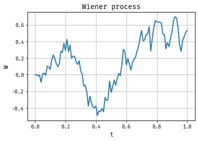
Figure 3: A Wiener Process
The upshot of all this is that the sum \[ \frac{1}{T} \sum_{t=1}^t y_{t-1} \epsilon_t \] convergences to a stochastic integral. Thus, suppose that \(y_t = y_{t-1} + \epsilon_t\), where \(\epsilon_t \stackrel{i.i.d.}{\sim} (0,\sigma^2)\) and \(y_0=0\). Then \[ \frac{1}{\sigma^2 T} \sum y_{t-1} \epsilon_t \Longrightarrow \int W(s) dW(s). \] where \(W(s)\) denotes a standard Wiener process. We can use this to develop tests!
Asymptotic Theory for Unit Root Process. Suppose that \(y_t = \phi y_{t-1} + \epsilon_t\), where \(\epsilon_t \sim iid(0,\sigma^2)\), \(\phi=1\), and \(y_0=0\). The sampling distribution of the OLS estimator \(\hat{\phi}_T\) of the autoregressive parameter \(\phi=1\) and the sampling distribution of the corresponding \(t\)-statistic have the following asymptotic approximations
\begin{eqnarray} z(\hat{\phi}_T) & \Longrightarrow & \frac{\frac{1}{2} ( W(1)^2 -1 ) }{ \int_0^1 W(s)^2 ds } \\ t(\hat{\phi}_T) & \Longrightarrow & \frac{\frac{1}{2} ( W(1)^2 -1 ) }{ \left[ \int_0^1 W(s)^2 ds \right]^{1/2} } \end{eqnarray}
where \(W(s)\) denotes a standard Wiener process.
To see these asymptotics, consider the simplified model \(y_t = \phi y_{t-1} + u_t\). We’ll try to estimation \(\phi\) by regression \(y_t\) on \(y_{t-1}\) (omitting the constant term.) Let’s consider two cases for the true value of \(\phi \in \{0.95, 1\}\). For each value of \(\phi\), we simulate many time series of length \(T = 5000\) and estimate \(\phi\) via OLS.
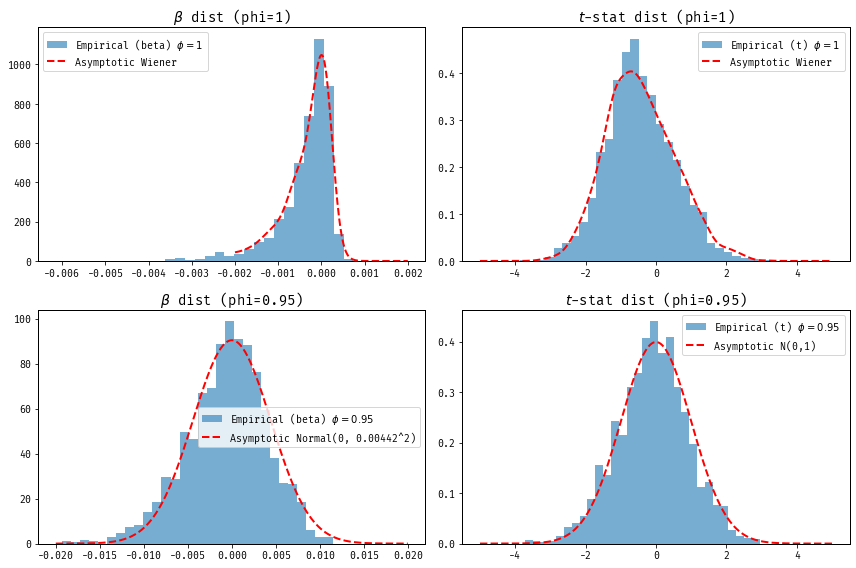
In practice, testing for a unit root in time series data uses results along these lines, with the specific critical values tabulated for the way lags of \(y_t\) enters the regression. You may have heard of Dickey-Fuller and Augmented Dickey-Fuller tests, the “augmented” refers to the inclusion of lagged differences of the time series as additional regressors to account for higher-order serial correlation, thus improving test performance in the presence of autocorrelated disturbances.
Replicating Nelson and Plosser (1982)
Nelson and Plosser (1982) investigate whether a set of key macroeconomic time series exhibited were better described by deterministic or stochastic trend models. We’ll return to the example in Figure 1 and focus on log Real GNP from 1909-1970. They first examine the estimated autocorrelation functions of the level and deviations from the time trend, both plotted in Figure 1:
These look pretty good, in the sense that the autocorrelations for the fluctuations (after removing the time trend) die out quickly, with a barely positive autocorrelation after the six lag. Unfortunately, as Nelson and Plosser (1982) point out, these estimated autocorrelations are also consistent with an integrated series. These kinds of statisical calculations often give misleading results (as we have just seen) when the underlying series is integrated.
To distinguish between the two trend paradigms, Nelson and Plosser (1982) decide to run the regression \[ y_t = \mu + \phi_1 y_{t-1} + \gamma t + \sum_{k=1}^K \phi_{\Delta k}\Delta y_{t-k} + u_t. \] They are interested in testing \(H_0: \phi_1 = 1, \gamma = 0\), and use the results from Dickey-Fuller to construct critical values. For log Real GNP, they set \(K = 2\). The results of the regression can be seen below.
These results match the first row of Table 5 in Nelson and Plosser (1982). The t-stat of \(-2.99\) would indicate that one should reject the marginal hypothesis that \(\phi_1 = 1\) at conventional significane levels. But these critical values are invalid in the unit root context. Instead the, say, 5 percent critial value tabulated by Dickey and Fuller is about \(-3.5\). Thus, one cannot reject the null that real GNP is well described by a unit root process.
Cointegrated Processes
We are often concerned with trending behavior for more than a single time series. For example, consider a bivariate model with a common stochastic trend:
\begin{eqnarray} y_{1,t} & = & \gamma y_{2,t} + u_{1,t} \\ y_{2,t} & = & y_{2,t-1} + u_{2,t} \end{eqnarray}
where \([u_{1,t}, u_{2,t}]’ \stackrel{i.i.d.}{\sim} iid(0,\Omega)\). Both \(y_{1,t}\) and \(y_{2,t}\) have a stochastic trend. However, there exists a linear combination of \(y_{1,t}\) and \(y_{2,t}\), namely, \[ y_{1,t} - \gamma y_{2,t} = u_t \] that is stationary. Therefore, \(y_{1,t}\) and \(y_{2,t}\) are called cointegrated. These profilerate in macro. Consider the RBC model:
\begin{eqnarray} \max_{\{c_t,k_t\}} \mathbb E_0\left[\sum_{t=0}^\infty \beta^t \ln c_t \right] \end{eqnarray}
subject to
\begin{eqnarray*} y_t &=& c_t + k_t = A^{1-\alpha} k_{t-1}^\alpha \\ \ln A_t &=& \gamma + \ln A_{t-1} + \epsilon_t. \end{eqnarray*}
Tedious algebra yields: \[ \ln y_t = -\frac{\alpha\gamma}{1-\alpha} + \ln A_t \text{ and } \ln c_t = \ln\left(1-\beta \alpha) y_t . \] Thus, \(y_t\) and \(c_t\) both inherit the stochastic trend in \(\ln A_t\). Back to our statistical framework. Clearly, \(y_{2,t}\) is a random walk. Moreover, it can be easily verified that \(y_{1,t}\) follows a unit root process.
\begin{eqnarray} y_{1,t} - y_{1,t-1} = \gamma (y_{2,t} - y_{2,t-1}) + u_{1,t} - u_{1,t-1} \end{eqnarray}
Therefore,
\begin{eqnarray} y_{1,t} = y_{1,t-1} + \gamma u_{2,t} + u_{1,t} - u_{1,t-1} \end{eqnarray}
Thus, both \(y_{1,t}\) and \(y_{2,t}\) are integrated processes. The vector \([1,-\gamma]’\) is called the cointegrating vector. Note that the cointegrating vector is only unique up to normalization. We’ll talk more about estimating these models once we’ve discussed vector autoregressions.