Bayesian VARs

Now we’re going to start putting things together to learn to estimate a cornerstone (Bayesian) model of macroeconomics, the autoregression (VAR.) VARs were first introduced to macroeconomics by Christopher A. Sims in Sims (1980) in an extremely important paper: “Macroeconomics and Reality.” Sims attacked the prevailing macroeconometric models of the day—including those used at the pFed—which featured systems of equations with many coefficients imposed, often as a zero. These models were estimated equation-by-equation, and often gave a (false) impression of both estimation precision and about the importance of particular transmission channels. Sims instead used a flexible VAR which modeled the contemporaneous and dynamic depedence for a time series of \(n\) variables \(y_t\). The VAR of order \(p\) follows the set of linear difference equations:

\begin{align} y_t = \Phi_0 + \Phi_1 y_{t-1} + \ldots + \Phi_p y_{t-p} + u_t. \end{align}

The innovations of \(u_t\) strictly speaking need only be white noise, but we’ll assume that they are independently and identically multivariate normally distributed,

\begin{align} u_t \stackrel{i.i.d.}{\sim} \mathcal N\left(0, \Sigma\right). \end{align}

So the VAR(\(p\)) mimics the previously discussed AR(\(p\)) with the difference being that \(y_t\) is now an \(n\times 1\) vector rather than a scalar.

Multivariate Time Series Basics

For theoretical analysis, it is often convenient to express the VAR(p) in the so-called companion form.

\begin{eqnarray} \hspace*{-0.5in} \left[ \begin{array}{c} y_t \\ y_{t-1} \\ \vdots \\ y_{t-p+1} \end{array} \right] = \left[ \begin{array}{c} \Phi_0 \\ 0 \\ \vdots \\ 0 \end{array} \right]

• \left[ \begin{array}{ccccc} \Phi_1 & \Phi_2 & \cdots & \Phi_{p-1} & \Phi_p \\ I & 0 & \cdots & 0 & 0 \\ \vdots & \vdots & \ddots & 0 & 0 \\ 0 & 0 & \cdots & I & 0 \end{array} \right] \left[ \begin{array}{c} y_{t-1} \\ y_{t-2} \\ \vdots \\ y_{t-p} \end{array} \right] + \left[ \begin{array}{c} u_t \\ 0 \\ \vdots \\ 0 \end{array} \right] \label{e_varcomp} \nonumber \end{eqnarray}

Let \(\xi_t = [y_t’, y_{t-1}’, \ldots, y_{t-p+1}’]’\). The VAR can be rewritten as

\begin{eqnarray} \xi_t = F_0 + F_1 \xi_{t-1} + \nu_t \end{eqnarray}

where the definitions of \(F_0\), \(F_1\), and \(\nu_t\) can be deduced from the previous equation. We have transformed our VAR(\(p\)) into a first-order vector autoregression (VAR(1)) in the companion form. We can easy recover the original time series by defining the \(n \times np\) matrix \(M_n = [I,0]\) where \(I\) is an \(n \times n\) identity matrix, so that \(y_t = M_n \xi_t\). The companion form is useful in two respects: (1) to define stationarity in the context of a VAR; (2) to convince ourselves that without loss of much generality we can restrict econometric analyses to VAR(1) specifications.

Result For a vector autoregression to be covariance stationary it is necessary that all eigenvalues of the matrix \(F_1\) are less than one in absolute value. \(\Box\)

Example

Consider the univariate AR(2) process \[ y_t = \phi_1 y_{t-1} + \phi_2 y_{t-2} + u_t \] The AR(2) process can be written in companion form as a VAR(1) where \(\xi_t = [y_t , y_{t-1}]’\) and \[ F_1 = \left[ \begin{array}{cc} \phi_1 & \phi_2 \\ 1 & 0 \end{array} \right] \] The eigenvalues \(\lambda\) of the matrix \(F_1\) satisfy the condition \[ det( F_1 - \lambda I) = 0 \iff (\phi_1 - \lambda)(-\lambda) - \phi_2 = 0 \] Provided that \(\lambda \not= 0\) the equation can be rewritten as \[ 0 = 1 - \phi_1 \frac{1}{\lambda} - \phi_2 \frac{1}{\lambda^2} \] Thus, the condition \(|\lambda| < 1\) is, at least in this example, equivalent to the condition that all the roots of the polynomial \(\phi(z)\) are greater than one in absolute value. A generalization of this example can be found in Hamilton (1994, Chapter 1). \(\Box\)

Describing a Covariance Stationary VAR(p) Process

Consider a VAR(p). The expected value of \(y_t\) has to satisfy the vector difference equation

\begin{eqnarray} {\mathbb E}[y_t] = \Phi_0 + \Phi_1 {\mathbb E}[y_{t-1}] + \ldots \Phi_p {\mathbb E}[y_{t-p}] \quad \mbox{for all} \; t \end{eqnarray}

If the eigenvalues of \(F_1\) are all less than one in absolute values and the VAR was initialized in the infinite past, then the expected value is given by

\begin{eqnarray} {\mathbb E}[y_t] = [ I - \Phi_1 - \ldots \Phi_t]^{-1} \Phi_0 \end{eqnarray}

To calculate the autocovariances we will assume that \(\Phi_0 = 0\). Consider the companion form

\begin{eqnarray} \xi_t = F_1 \xi_{t-1} + \nu_t \end{eqnarray}

If the eigenvalues of \(F_1\) are all less than one in absolute value and the VAR was initialized in the infinite past, than the autocovariance matrix of order zero has to satisfy the equation

\begin{eqnarray} \Gamma_{\xi \xi,0} = {\mathbb E}[\xi_t \xi_t’] = F_1 \Gamma_{\xi \xi,0} F_1’ + {\mathbb E}[ \nu_t \nu_t’] \end{eqnarray}

Obtaining a closed form solution for \(\Gamma_{\xi \xi,0}\) is a bit more complicated than in the univariate AR(1) case.

Some Facts

\begin{definition} Let $A$ and $B$ be $2 \times 2$ matrices with the elements \[ A = \left[ \begin{array}{cc} a_{11} & a_{12} \\ a_{21} & a_{22} \end{array} \right], \quad B = \left[ \begin{array}{cc} b_{11} & b_{12} \\ b_{21} & b_{22} \end{array} \right] \] The $vec$ operator is defined as the operator that stacks the columns of a matrix, that is, \[ vec(A) = [ a_{11}, a_{21}, a_{12}, a_{22} ]' \] and the Kronecker product is defined as \[ A \otimes B = \left[ \begin{array}{cc} a_{11}B & a_{12}B \\ a_{21}B & a_{22}B \end{array} \right] \quad \Box \] \end{definition}

\begin{lemma} Let $A$, $B$, $C$ be matrices whose dimension are such that the product $ABC$ exists. Then $vec(ABC) = (C’ \otimes A)vec(B) \quad \Box$ \end{lemma}

A closed form solution for the elements of the covariance matrix of \(\xi_t\) can be obtained as follows

\begin{eqnarray} vec(\Gamma_{\xi \xi,0}) & = &(F_1 \otimes F_1) vec(\Gamma_{\xi\xi,0}) + vec( {\mathbb E}[\nu_t \nu_t’] ) \nonumber \\ & = & [ I - (F_1 \otimes F_1)]^{-1} vec( {\mathbb E}[\nu_t \nu_t’] ) \end{eqnarray}

Since

\begin{eqnarray} {\mathbb E}[ \xi_t \xi_{t-h}’ ] = F {\mathbb E}[\xi_{t-1} \xi_{t-h}’] + {\mathbb E}[\nu_t \xi_{t-h}’] \end{eqnarray}

we can deduce that

\begin{eqnarray} \Gamma_{\xi \xi,h} = F^h_1 \Gamma_{\xi \xi,0} \end{eqnarray}

To obtain the autocovariance \(\Gamma_{\xi \xi,-h}\) we have to keep track of a transpose in the general matrix case:

\begin{eqnarray} \Gamma_{\xi \xi,-h} = {\mathbb E}[ \xi_{t-h} \xi_t’ ] = \bigg[ {\mathbb E}[ \xi_t \xi_{t-h}’] \bigg]’ = \Gamma_{\xi \xi,h}' \end{eqnarray}

Once we have calculate that autocovariances for the companion form process \(\xi_t\) it is straightforward to obtain the autocovariances for the \(y_t\) process. Since \(y_t = M_n \xi_t\) it follows that

\begin{eqnarray} \Gamma_{yy,h} = {\mathbb E}[y_t y_{t-h}’] = {\mathbb E}[ M_n \xi_t \xi_{t-h}’ M_n’] = M_n \Gamma_{\xi \xi,h} M_n' \end{eqnarray}

Result: Consider the vector autoregression \[ y_t = \Phi_0 + \Phi_1 y_{t-1} + \ldots + \Phi_p y_{t-p} + u_t \] where \(u_t \sim iid {\cal N}(0,\Sigma)\) with companion form \[ \xi_t = F_0 + F_1 \xi_{t-1} + \nu_t \] Suppose that the eigenvalues of \(F_1\) are all less than one in absolute values and that the vector autoregression was initialized in the infinite past. Under these assumptions the vector process \(y_t\) is covariance stationary with the moments

\begin{eqnarray} {\mathbb E}[y_t] & = & [ I - \Phi_1 - \ldots \Phi_t]^{-1} \Phi_0 \\ \Gamma_{yy,h} & = & M_n \Gamma_{\xi \xi,h} M_n’ \quad \forall h \end{eqnarray}

where

\begin{eqnarray} vec(\Gamma_{\xi\xi,0}) & = & [ I - (F_1 \otimes F_1)]^{-1} vec( {\mathbb E}[\nu_t \nu_t’] ) \\ \Gamma_{\xi \xi,h} & = & F_1^h \Gamma_{\xi \xi,0} \quad h > 0 \quad \Box \end{eqnarray}

The Likelihood of a VAR(p)

We will now derive the likelihood function for a Gaussian VAR(p), conditional on initial observations \(y_0, \ldots, y_{-p+1}\). The density of \(y_t\) conditional on \(y_{t-1}, y_{t-2}, \ldots\) and the coefficient matrices \(\Phi_0, \Phi_1, \ldots, \Sigma\) is of the form

\begin{eqnarray} \hspace*{-0.5in} p(y_t|Y^{t-1}, \Phi_0, \ldots, \Sigma) &\propto& |\Sigma|^{-1/2} \exp \bigg\{ - \frac{1}{2} ( y_t - \Phi_0 - \Phi_1 y_{t-1} - \ldots - \Phi_p y_{t-p} )’ \nonumber \\ &~& \times \Sigma^{-1} ( y_t - \Phi_0 - \Phi_1 y_{t-1} - \ldots - \Phi_p y_{t-p} ) \bigg\} \end{eqnarray}

Define the \((np+1) \times 1\) vector \(x_t\) as \[ x_t = [ 1, y_{t-1}’, \ldots, y_{t-p}’]' \] Moreover, define the matrixes \[ Y = \left[ \begin{array}{c} y_1’ \\ \vdots \\y_T’ \end{array} \right], \quad X = \left[ \begin{array}{c} x_1’ \\ \vdots \\x_T’ \end{array} \right], \quad \Phi = [ \Phi_0, \Phi_1, \ldots, \Phi_p]' \] The conditional density of \(y_t\) can be written in more compact notation as

\begin{eqnarray} p(y_t| Y^{t-1}, \Phi, \Sigma) \propto |\Sigma|^{-1/2} \exp \left\{ - \frac{1}{2} ( y_t’ - x_t’\Phi ) \Sigma^{-1} ( y_t’ - x_t’\Phi )’ \right\} \end{eqnarray}

To manipulate the density we will use some matrix algebra facts.

Facts:

1. Let \(a\) be a \(n \times 1\) vector, \(B\) be a symmetric positive definite \(n \times n\) matrix, and \(tr\) the trace operator that sums the diagonal elements of a matrix. Then \[ a’Ba = tr[Baa’] \]
2. Let \(A\) and \(B\) be two \(n \times n\) matrices, then \[ tr[A+B] = tr[A] + tr[B] \]

In a first step, we will replace the inner product in the expression for the conditional density by the trace of the outer product

\begin{eqnarray} p(y_t| Y^{t-1}, \Phi, \Sigma) \propto |\Sigma|^{-1/2} \exp \left\{ - \frac{1}{2} tr[ \Sigma^{-1}( y_t’ - x_t’\Phi )’( y_t’ - x_t’\Phi )] \right\} \end{eqnarray}

In the second step, we will take the product of the conditional densities of \(y_1, \ldots, y_T\) to obtain the joint density. Let \(Y_0\) be a vector with initial observations

\begin{eqnarray} p(Y|\Phi,\Sigma, Y_0) &=& \prod_{t=1}^T p(y_t|Y^{t-1}, Y_0, \Phi, \Sigma) \nonumber \\ &\propto& |\Sigma|^{-T/2} \exp \left\{ -\frac{1}{2} \sum_{t=1}^T tr[\Sigma^{-1}( y_t’ - x_t’\Phi )’( y_t’ - x_t’\Phi )] \right\} \nonumber \\ &\propto& |\Sigma|^{-T/2} \exp \left\{ -\frac{1}{2} tr\left[\Sigma^{-1}\sum_{t=1}^T( y_t’ - x_t’\Phi )’( y_t’ - x_t’\Phi )\right] \right\} \nonumber \\ &\propto& |\Sigma|^{-T/2} \exp \left\{ -\frac{1}{2} tr [ \Sigma^{-1} (Y-X\Phi)’(Y-X\Phi) ] \right\} \end{eqnarray}

Define the ``OLS’’ estimator

\begin{eqnarray} \hat{\Phi} = (X’X)^{-1} X’Y \end{eqnarray}

and the sum of squared OLS residual matrix

\begin{eqnarray} S = (Y - X \hat{\Phi})’(Y- X \hat{\Phi}) \end{eqnarray}

It can be verified that

\begin{eqnarray} (Y - X\Phi)’(Y-X\Phi) = S + (\Phi - \hat{\Phi})‘X’X(\Phi- \hat{\Phi}) \end{eqnarray}

Problem: Verify this!

x = 1

This leads to the following representation of the likelihood function

\begin{eqnarray} p(Y|\Phi,\Sigma, Y_0) &\propto& |\Sigma|^{-T/2} \exp \left\{ -\frac{1}{2} tr[\Sigma^{-1} S] \right\}\nonumber \\ &~&\times \exp \left\{ -\frac{1}{2} tr[ \Sigma^{-1}(\Phi - \hat{\Phi})‘X’X(\Phi- \hat{\Phi})] \right\} \end{eqnarray}

An Alternative Representation

Let \(\beta = vec(\Phi)\) and \(\hat{\beta} = vec(\hat{\Phi})\). It can be verified that

\begin{eqnarray} tr[ \Sigma^{-1}(\Phi - \hat{\Phi})‘X’X(\Phi- \hat{\Phi})] = (\beta - \hat{\beta})’[ \Sigma \otimes (X’X)^{-1} ]^{-1} (\beta - \hat{\beta}) \end{eqnarray}

and the likelihood function has the alternative representation

\begin{eqnarray} p(Y|\Phi,\Sigma, Y_0) &\propto& |\Sigma|^{-T/2} \exp \left\{ -\frac{1}{2} tr[\Sigma^{-1} S] \right\} \nonumber \\ &~&\times \exp \left\{ -\frac{1}{2} (\beta - \hat{\beta})’[ \Sigma \otimes (X’X)^{-1} ]^{-1} (\beta - \hat{\beta}) \right\} \nonumber \end{eqnarray}

Bayesian Inference

Before we do Bayesian inference we need to get some multivariate statistical tools.

The Inverse Wishart Distribution (wikipedia)

We need to think about probability distributions of \(\Sigma\). This a little complicated because the space of admissible (positive definite) covariance matrix is a particular manifold inside \(\mathbb R^{n^2}\). Luckily, there exists such a probability distribution, called the inverse Wishart distribution. This distribution is the multivariate version of the inverted gamma distribution. Let \(W\) be a \(n \times n\) positive definite random matrix. \(W\) has the inverted Wishart \(IW(S,\nu)\) distribution if its density is of the form

\begin{eqnarray} p(W|S,\nu) \propto |S|^{\nu/2} |W|^{-(\nu+n+1)/2}\exp \left\{ - \frac{1}{2} tr[W^{-1}S] \right\} \end{eqnarray}

The Wishart distribution arises in the Bayesian analysis of multivariate regression models. To sample a \(W\) from an inverted Wishart \(IW(S,\nu)\) distribution, draw \(n \times 1\) vectors \(Z_1,\ldots, Z_\nu\) from a multivariate normal \({\cal N}(0,S^{-1})\) and let \[ W = \left[ \sum_{i=1}^\nu Z_iZ_i’\right]^{-1} \] Note: to generate a draw \(Z\) from a multivariate \({\cal N}(\mu,\Sigma)\), decompose \(\Sigma = CC’\), where \(C\) is the lower triangular Cholesky decomposition matrix. Then let \(Z = \mu + C {\cal N}(0,{\cal I})\).

Caution. The inverse Wishart distribution has haters on the internet.

Matrix Normal Distribution (wikipedia)

Let \(Z\) by a \(T \times n\) matrix. \(Z\) follows a matrix normal distribution with parameters \(\Mu\) (an \(T\times n\) matrix), \(\Sigma\) (an \(n \times n\) positive definite matrix), and \(\Omega\) (a \(T \times T\) positive definite matrix), if it has density:

\begin{align} p(Z|M, \Sigma, \Omega) = (2\pi)^{-Tn/2} |\Sigma|^{-T/2} |\Omega|^{-n/2} \exp\left\{-\frac12\mbox{tr}(\Sigma^{-1} (Z - M)’ \Omega^{-1} (Z - M))\right\}. \end{align}

If \(Z\) follows a matrix normal distribution, then \(vec(Z)\) follows a multivariate normal distribution with mean \(vec(M)\) and variance \(\Omega \otimes \Sigma\). To see this note that the term in the exponent can be rewritten as:

\begin{align} \mbox{tr}(\Sigma^{-1} (Z - M)’ \Omega^{-1} (Z - M)) & = vec\left((Z - M)\Sigma^{-1} \right)’ vec\left(\Omega^{-1} (Z - M) \right) \nonumber \\ & = \left[ \left(\Sigma^{-1} \otimes I_T \right)vec\left(Z - M\right) \right]’ \left[ \left(I_n \otimes \Omega^{-1} \right) vec\left(Z - M\right)\right] \nonumber \\ & = vec\left(Z-M\right)’\left(\Sigma^{-1} \otimes I_T \right) \left(I_n \otimes \Omega^{-1} \right)vec\left(Z - M\right) \nonumber \\ &= \left(vec(Z) - vec(M)\right)’\left(\Sigma \otimes \Omega \right)^{-1} \left(vec(Z) - vec(M)\right) \end{align}

and also noting that \(|\Sigma|^{T}|\Omega|^{n} = |\Sigma \otimes \Omega|\). Often \(\Omega\) is called the “among row” covariance matrix and \(\Sigma\) is called the “among column” covariance matrix. So increasing \(\Sigma_{1,1}\) will increase the variance of \(Z_{\cdot1}\) and increasing \(\Sigma_{1,2}\) with increase the covariance between \(Z_{\cdot1}\) and \(Z_{\cdot2}\).

The Likelihood of VAR(p) As A Matrix Normal

Let’s consider a VAR with \(n\) variables \( (y_t\) is \(n\times 1)\) and \(p\) lags.

\begin{align} y_t = \Phi_0 + \Phi_1 y_{t-1} + \ldots + \Phi_p y_{t-p} + u_t, \quad u_t \sim N\left(0,\Sigma\right). \end{align}

Let \(x_t = [1,y_{t-1}’,\ldots,y_{t-p}’]’\) and \(\Phi = [\Phi_0,\Phi_1,\ldots,\Phi_p]\): \[ y_t’ = x_t’\Phi + u_t’ \] Let,

\begin{align} Y = \left[\begin{array}{c} y_1’ & \vdots & y_T’ \end{array}\right], X = \left[\begin{array}{c} x_1’ & \vdots & x_T’ \end{array}\right], \mbox{ and } U = \left[\begin{array}{c} u_1’ & \vdots & u_T’ \end{array}\right]. \end{align}

We have

\begin{align} Y = X \Phi + U. \end{align}

Notice that the columsn of \(U\) has a covariance determined by \(\Sigma\), while the rows are independent. So \(U\) follows a matrix normal distribution with mean zero and covariance parameters \(\Sigma\) and \(I_T\). Thus, \(Y\) follows a matrix normal distribution with likelihood given by:

\begin{align} p(Y|\Phi,\Sigma) = (2\pi)^{-np/2} |\Sigma|^{-T/2} \exp\left\{-\frac12 tr\left[\Sigma^{-1} \left(Y-X\Phi\right)’\left(Y - X\Phi\right)\right]\right\}. \end{align}

Dummy Observation Priors

VARs are very flexible time series models, but their flexiblity comes at a cost. The Bayesian paradigm is especially well suited

There are many ways to structure prior distributions for VARs. Here we’ll talk about using pseudo-data, also known as dummy observations. Suppose we have \(T^*\) dummy observations \((Y^*,X^*)\). The likelihood function for the dummy observations is of the form

\begin{eqnarray} \lefteqn{ p( Y^* | \Phi,\Sigma ) = (2 \pi)^{-nT^*/2} |\Sigma|^{- T^*/2}} \label{eq_priordummy1} \\ && \exp \left\{ - \frac{1}{2} tr[ \Sigma^{-1}(Y^{*’}Y^* - \Phi’X^{*’}Y^* - Y^{*’}X^{*} \Phi + \Phi’ X^{*’}X^* \Phi)] \right\}. \nonumber \end{eqnarray}

Combining~(\ref{eq_priordummy1}) with the improper prior \(p(\Phi,\Sigma) \propto | \Sigma|^{-(n+1)/2}\) yields

\begin{eqnarray} \hspace*{-0.6in} p(\Phi,\Sigma | Y^*) &=& c_*^{-1} | \Sigma|^{- \frac{ T^*+n+1}{2}}\nonumber \\ &~& exp \left\{ - \frac{1}{2} tr[ \Sigma^{-1}(Y^{*’}Y^* - \Phi’X^{*’}Y^* - Y^{*’}X^{*} \Phi + \Phi’ X^{*’}X^* \Phi)] \right\},\nonumber \end{eqnarray}

which can be interpreted as a prior density for \(\Phi\) and \(\Sigma\).

Define

\begin{eqnarray*} \hat{\Phi}^* &=& (X^{*’}X^*)^{-1}X^{*’}Y^* \\ S^* &=& (Y^* - X^* \hat{\Phi}^*)’(Y^* - X^* \hat{\Phi}^*). \end{eqnarray*}

It can be verified that the prior \(p(\Phi,\Sigma | Y^*)\) is of the Inverted Wishart-Normal \({\cal IW}-{\cal N}\) form

\begin{eqnarray} \Sigma & \sim & {\cal IW} \bigg( S^*, T^*-k \bigg) \\ \Phi | \Sigma & \sim & {\cal N} \bigg( \Phi^*, \Sigma \otimes (X^{*’} X^{*})^{-1} \bigg). \end{eqnarray}

Problem: Verify this!

x = 1

The appropriate normalization constant for the prior density is given by

\begin{eqnarray} c_* &=& (2 \pi)^{\frac{nk}{2}} | X^{*’}X^*|^{-\frac{n}{2}} | S^*|^{- \frac{ T^* -k}{2} } \\ && 2^{\frac{n(T^* -k)}{2}} \pi^{ \frac{n(n-1)}{4} } \prod_{i=1}^n \Gamma[(T^* - k+1 - i)/2], \nonumber \end{eqnarray}

\(k\) is the dimension of \(x_t\) and \(\Gamma[\cdot]\) denotes the gamma function.

Problem: Verify this!

x = 1

Details of this calculation can be found in cite:zellner1971. The implementation of priors through dummy variables is often called mixed estimation and dates back to Theil and Goldberger (1961).

Timeline of the Minnesota Prior GLP

The baseline prior is a version of the so-called Minnesota prior, first introduced in Litterman (1979) and later refined in Litterman (1980).

The first prior of this type is known as “sum-of-coefficients” prior and was originally proposed by cite:Doan1984

cite:sims1993nine known as “dummy-initial-observation”

his deterministic component is defined as τt ≡ Ep ( yt|y1, …, yp, ˆβ ) , i.e. the expectation of future y’s given the initial conditions and the value of the estimated VAR coefficients. According to cite:sims1992bayesian, in un- restricted VARs, τt has a tendency to exhibit temporal heterogeneity—a markedly different behavior at the beginning and the end of the sample—and to explain an im- plausibly high share of the variation of the variables over the sample.

Minnesota Prior

VARs really began to take off for forecasting and other purposes when combined with Bayesian methods. The reason why Bayes is so helpful is that VARs contain a lot of parameters, and we don’t have (relatively speaking) a lot of aggregate macroeconomic data. So frequentist methods tended to overfit and make poor out of sample predictions. A prior distribution for Bayesian VARs which avoided this problem was developed in the early 1980s by researchers at the University of Minnesota and the Federal Reserve Bank of Minneapolis, dubbed the Minnesota Prior. It can be implemented using dummy observations. What follows is a brief description, see Doan, Litterman, and Sims (1984) for details.

Consider the following Gaussian bivariate VAR(2).

\begin{eqnarray} \hspace{-0.5in} \left[ \begin{array}{c} y_{1,t} \\ y_{2,t} \end{array} \right] = \left[ \begin{array}{c} \alpha_1 \\ \alpha_2 \end{array} \right] + \left[ \begin{array}{cc} \beta_{11} & \beta_{12} \\ \beta_{21} & \beta_{22} \end{array} \right] \left[ \begin{array}{c} y_{1,t-1} \\ y_{2,t-1} \end{array} \right] + \left[ \begin{array}{cc} \gamma_{11} & \gamma_{12} \\ \gamma_{21} & \gamma_{22} \end{array} \right] \left[ \begin{array}{c} y_{1,t-2} \\ y_{2,t-2} \end{array} \right] + \left[ \begin{array}{c} u_{1,t} \\ u_{2,t} \end{array} \right] \end{eqnarray}

Define \(y_t = [y_{1,t}, y_{2,t}]’\), \(x_t = [y_{t-1}’, y_{t-2}’,1]’\), and \(u_t = [ u_{1,t}, u_{2,t}]’\) and

\begin{eqnarray} \Phi = \left[ \begin{array}{cc} \beta_{11} & \beta_{21} \\ \beta_{12} & \beta_{22} \\ \gamma_{11} & \gamma_{21} \\ \gamma_{12} & \gamma_{22} \\ \alpha_1 & \alpha_2 \end{array} \right]. \end{eqnarray}

The VAR can be rewritten as follows

\begin{eqnarray} y_t’ = x_t’ \Phi + u_t’ , \quad t=1,\ldots,T, \quad u_t \sim iid{\cal N}(0,\Sigma) \end{eqnarray}

or in matrix form

\begin{eqnarray} Y = X \Phi + U. \end{eqnarray}

Based on a short pre-sample \(Y_0\) (typically the observations used to initialized the lags of the VAR) one calculates: \(s = std(Y_0)\) and \(\bar{y} = mean(Y_0)\). In addition there are a number of tuning parameters for the prior

• \(\tau\) is the overall tightness of the prior. Large values imply a small prior covariance matrix.
• \(d\): the variance for the coefficients of lag \(h\) is scaled down by the factor \(l^{-2d}\).
• \(w\): determines the weight for the prior on \(\Sigma\). Suppose that \(Z_i = {\cal N}(0,\sigma^2)\). Then an estimator for \(\sigma^2\) is \(\hat{\sigma}^2 = \frac{1}{w} \sum_{i=1}^w Z_i^2.\) The larger \(w\), the more informative the estimator, and in the context of the VAR, the tighter the prior.
• \(\lambda\) and \(\mu\): additional tuning parameters.

Dummies for the \(\beta\) coefficients: \[ \left[ \begin{array}{cc} \tau s_1 & 0 \\ 0 & \tau s_2 \end{array} \right] = \left[ \begin{array}{ccccc} \tau s_1 & 0 & 0 & 0 & 0 \\ 0 & \tau s_2 & 0 & 0 & 0 \end{array} \right] \Phi + u’ \] The first observation implies, for instance, that \hspace{-0.50in}

\begin{eqnarray*} \hspace{-0.50in} \tau s_1 &=& \tau s_1 \beta_{11} + u_1 \quad \Longrightarrow \beta_{11} = 1 - \frac{u_1}{\tau s_1} \quad \Longrightarrow \quad \beta_{11} \sim {\cal N} \left( 1, \frac{\Sigma_{u,11}}{\tau^2 s_1^2} \right) \\ 0 &=& \tau s_1 \beta_{21} + u_2 \quad \Longrightarrow \beta_{21} = - \frac{u_2}{\tau s_1} \quad \Longrightarrow \quad \beta_{21} \sim {\cal N} \left( 0, \frac{\Sigma_{u,22}}{\tau^2 s_1^2} \right) \end{eqnarray*}

Dummies for the \\(\gamma\\) coefficients

\[ \left[ \begin{array}{cc} 0 & 0 \\ 0 & 0 \end{array} \right] = \left[ \begin{array}{ccccc} 0 & 0 & \tau s_1 2^d & 0 & 0 \\ 0 & 0 & 0 & \tau s_2 2^d & 0 \end{array} \right] \Phi + u' \] The prior for the covariance matrix is implemented by \[ \left[ \begin{array}{cc} s_1 & 0 \\ 0 & s_2 \end{array} \right] = \left[ \begin{array}{ccccc} 0 & 0 & 0 & 0 & 0 \\ 0 & 0 & 0 & 0 & 0 \end{array} \right] \Phi + u' \]

                     Co-persistence prior dummy observations, reflecting the belief that
  when data on all \\(y\\)'s are stable at their initial levels, thy will
  tend to persist at that level:
  \\[
    \left[ \begin{array}{cc} \lambda \bar{y}\_1 & \lambda \bar{y}\_2
           \end{array} \right]
    = \left[ \begin{array}{ccccc} \lambda \bar{y}\_1 & \lambda \bar{y}\_2 & \lambda \bar{y}\_1 & \lambda \bar{y}\_2 & \lambda
             \end{array} \right] \Phi + u'
  \\]

Own-persistence prior dummy observations, reflecting the belief that when \(y_i\) has been stable at its initial level, it will tend to persist at that level, regardless of the value of other variables: \[ \left[ \begin{array}{cc} \mu \bar{y}_1 & 0 \\ 0 & \mu \bar{y}_2 \end{array} \right] = \left[ \begin{array}{ccccc} \mu \bar{y}_1 & 0 & \mu \bar{y}_1 & 0 & 0 \\ 0 & \mu \bar{y}_2 & 0 & \mu \bar{y}_2 & 0 \end{array} \right] \Phi + u' \]

In the same way we constructed a prior from dummy observations, we can also construct a prior from a training sample. Suppose we split the actual sample \(Y = [ Y^{-} , Y^{+} ]\), where \(Y^{-}\) is interpreted as training sample, then

\begin{eqnarray} \hspace*{-0.3in} p(\Phi,\Sigma) &=& c_-^{-1} | \Sigma|^{- \frac{ T^-+n+1}{2}}\nonumber\\ &~&\left\{ - \frac{1}{2} tr[ \Sigma^{-1}(Y^{-’}Y^- - \Phi’X^{-’}Y^- - Y^{-’}X^{-} \Phi + \Phi’ X^{-’}X^- \Phi)] \right\},\nonumber \end{eqnarray}

Of course one can also combine the dummy observations and training sample to construct a prior distribution.

Notice that

\begin{eqnarray} p(\Phi,\Sigma|Y) \propto p(Y|\Phi,\Sigma) p(Y^*|\Phi,\Sigma) \end{eqnarray}

Now define:

\begin{eqnarray} \tilde{\Phi} &=& (X^{*’}X^* + X’X)^{-1}(X^{*’}Y^* + X’Y) \label{eq_phitilde}\\ \tilde{\Sigma}_u &=& \frac{1}{T^*+ T} \bigg[ (Y^{*’}Y^* + Y’Y) \nonumber \\ && - (X^{*’}Y^* + X’Y)’(X^{*’}X^* + X’X)^{-1}(X^{*’}Y^* + X’Y) \bigg]. \label{eqa_sigtilde} \end{eqnarray}

Since prior and likelihood function are conjugate, it is straightforward to show, e.g., Zellner (1971), that the posterior distribution of \(\Phi\) and \(\Sigma\) is also of the Inverted Wishart – Normal form:

\begin{eqnarray} \Sigma | Y & \sim & {\cal IW} \bigg( (T^*+T) \tilde{\Sigma}_u,T^*+T-k\bigg) \label{eq_sigpost} \\ \Phi | \Sigma, Y & \sim & {\cal N} \bigg( \tilde{\Phi}, \Sigma \otimes (X^{*’}X^* + X’X)^{-1} \bigg). \label{eq_phipost} \end{eqnarray}

Suppose that we are using a prior constructed from a training sample and dummy observations. Then the marginal data density is given by

\begin{eqnarray} p(Y^+ | Y^-, Y^*, {\cal M}_0) = \frac{ \int p( Y^+, Y^-, Y^* | \Phi,\Sigma) d \Phi d\Sigma }{ \int p( Y^-, Y^* | \Phi,\Sigma) d \Phi d\Sigma } \end{eqnarray}

where the integrals in the numerator and denominator are given by the appropriate modification of \(c_*\) defined above. More specifically:

\begin{eqnarray} \hspace{-0.5in} \int p(Y | \Phi, \Sigma) d \Phi d\Sigma = \pi^{- \frac{T-k}{2}} | X’X |^{-\frac{n}{2}} | S|^{- \frac{ T -k}{2} } \pi^{ \frac{n(n-1)}{4} } \prod_{i=1}^n \Gamma[(T - k+1 - i)/2], \end{eqnarray}

where

\begin{eqnarray*} \hat{\Phi} &=& (X’X)^{-1}X’Y \\ S &=& (Y - X \hat{\Phi})’(Y - X \hat{\Phi}). \end{eqnarray*}

The Structural VAR

Let’s restrict to an \(n\) variable VAR(1) with mean zero for simplicity. The VAR model is given by

\begin{align} y_t = \Phi_1 y_{t-1} + u_t, \quad u_t \stackrel{i.i.d.}{\sim} {\cal N}(0,\Sigma) \end{align}

The vector \(u_t\) corresponds to the one-step-ahead forecast errors. Macroeconomic theory suggests that these forecast errors are driven by structural shocks, \(\epsilon_t\). We can write the VAR in structural form as

\begin{align} A_0 y_t = A_1 y_{t-1} + \epsilon_t, \quad \epsilon_t \stackrel{i.i.d.}{\sim} {\cal N}(0,I) \end{align}

One can think of the rows of \(A_0\) and \(A_1\) as corresponding the coefficients associated with a given equation of the equilibrium system implied by the VAR. Letting \(A_i = [a_{i,jk}]\) and setting \(A_1 = 0\)

\begin{align} a_{0,11} y_{t,1} + a_{0,12} y_{t,2} + \cdots + a_{0,1n} y_{t,n} &= \epsilon_{t,1} \\ a_{0,21} y_{t,1} + a_{0,22} y_{t,2} + \cdots + a_{0,2n} y_{t,n} &= \epsilon_{t,2} \\ & \vdots \\ a_{0,n1} y_{t,1} + a_{0,n2} y_{t,2} + \cdots + a_{0,nn} y_{t,n} &= \epsilon_{t,n} \end{align}

These equations describe the relationships among the variables in \(y_t\) in terms of the structural shocks \(\epsilon_t\). How does one estimate the relationships? Consider the relationship between the two VAR representations. Assuming \(A_0\) is invertible—invertibility here simply means…—it’s easy to go from \((A_0, A_1)\) to \((\Phi, \Sigma)\):

\begin{align} y_t = \underbrace{A_0^{-1} A_{1}}_{\Phi_1} y_{t-1} + \underbrace{A_0^{-1} \epsilon_t}_{u_t}, \mbox{ with } \Sigma = A_0^{-1} (A_0^{-1})' \end{align}

But the reverse is not so easy. Suppose one knows \(\Sigma\). We could consider taking \(A_0^{-1}\) to be the lower Cholesky decomposition of \(\Sigma\). We write this as \(A_0 = \text{chol}(\Sigma)^{-1}.\) This choice for \(A_0\) with of course satisfy \(\Sigma = A_0^{-1} (A_0^{-1})’\) by construction. But now consider an alternative choice \(\tilde A_0 = \text{chol}(\Sigma)^{-1}\Omega \), where \(\Omega\) is an orthonormal matrix. An orthonormal matrix \(\Omega\) has the property that \(\Omega’\Omega = I\), where \(I\) is the identity matrix. This implies that \(\Omega\) preserves the length of vectors it multiplies and its inverse is simply its transpose, i.e., \(\Omega^{-1} = \Omega’\). We have

\begin{align} \tilde A_0^{-1} (\tilde A_0^{-1})’ = A_0^{-1} \Omega^{-1} (\Omega^{-1})’ (A_0^{-1})’ = \Sigma. \end{align}

This is the fundamental identification problem associated with structural VARs. It is impossible to recover \((A_0, A_1)\) from \((\Phi, \Sigma)\). An immediate implication of [] is that \(p(Y|A_0, A_1) = p(Y|\tilde A_0, \tilde A_1)\). The identification can be understood from many different perspectives, but it is perhaps most simple to understand it as one of counting: there are \(n^2\) parameters in \(A_0\) but only \(n(n+1)/2\)—less than \(n^2\) if \(n>1\)—free parameters in the covariance matrix \(\Sigma\).

Identifying \(\Omega\)

In what follows we’ll discuss different identification strategies in the literature in with an emphasis on bivariate VARs. In general defining the space of orthogonal matrices is tedious, but for \(n = 2\) we can use a Givens matrix, which rotates vectors in a 2-dimensional plane. It has the form: \[ \Omega(\theta) = \begin{bmatrix} \cos(\theta) & -\sin(\theta) \\ \sin(\theta) & \cos(\theta) \end{bmatrix} \] Here, \(\theta\) is the rotation angle. It is trival to check that this matrix satisfies the orthonormality condition \(\Omega’\Omega = I\). As we discussed above, an identification scheme is simply a prior distribution \(p(\theta | \Phi, \Sigma)\). Note that in general \(\theta \in [-\pi, \pi]\).

Short Run Restrictions

The first kind of restriction is owing to Sims (1986). After arguing that VARs ought to be the benchmark time series model for macroeconomic analysis, Sims turned to the question of policy analysis. He argued for timing-based identification of \(A_0\), with an emphasis on lags in information as an identifying assumption. Here he writes:

… the idea that the monetary authority and the banks can see interest rates and indicators of movements in monetary aggregates immediately, but can only react to the remaining variables in the economy after a delay because data on these variables are released later.

This logic is extended beyond the policy variables (the interest rate and money supply) to the rest of the variables in his VAR. Ultimately, these timing assumptions lead to an \(A_0\) that is lower triangular with zeros in the upper right block. This identification is sometimes called “recursive” because it implies a sequential response structure where each variable can be contemporaneously influenced only by itself and preceding variables in the ordering, but not by those that follow. Sims calls this following the “Wold causal chain” highlighting how the shocks \(\epsilon_{i,t}\) associated with this approach can serve as the innovations in a Wold decomposition of the series.

In this identification scheme, it’s easy to recover \(A_0\) from \(\Sigma\). In the framework above, this amounts to setting \(\Omega = I.\) In our two variable setup this corresponds to a dogmatic prior on which concentrates \(\Omega\) on this matrix, i.e., \(\theta = 0\).

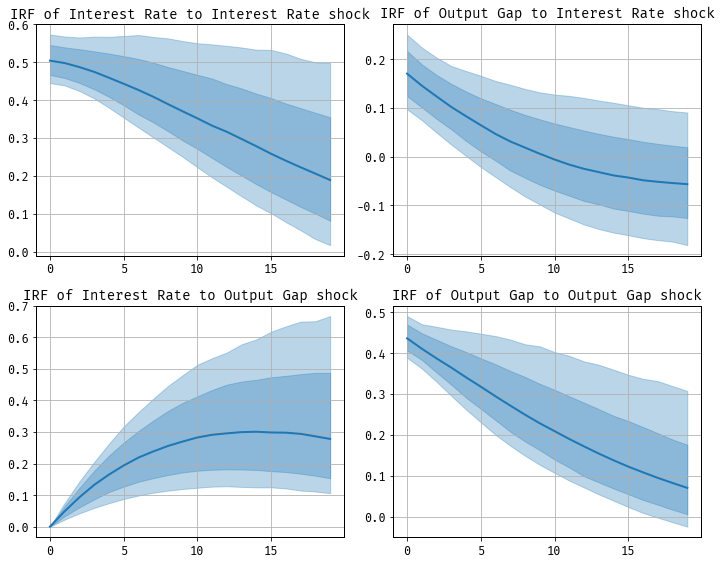
Example. Let’s consider the two variable VAR in the interest rate and the output gap, \(y_t = [i_t, x_t]’\). Our recursive identification scheme implies

\begin{align} a_{0, 11} i_t &= \text{… lags of \(i_t\) and \(x_t\) …} + \epsilon_{1,t} \\ a_{0, 21} i_t + a_{0, 22} x_t &= \text{… lags of \(i_t\) and \(x_t\) …} + \epsilon_{2,t} \end{align}

The interest rate \(i_t\) is contemporaneously unaffected by the output gap \(x_t\), but the output gap may respond immediately to changes in the interest rate. Typically, the first equation is interpeted as the policy equation—that is, the monetary policy reaction function. Here, monetary policy is a function of the lagged interest rate, the lagged output gap, and a shock \(\epsilon_{1,t}\). This shock is given the interpretation of a monetary policy shock and the impulse of the endogenous variables in the system is of great interest to economists.

A potential source of confusion is in myriad sets of notation used in the SVAR literature. Here we defined \(A_0\) as the matrix of contemporaneous relationships among the variables in the structural VAR. Some instead define \(A_0\) (labelled however) as the matrix that relates the structural shocks directly to the reduced-form errors, which is usually inverted compared to our definition. In this “impact matrix” formulation, \(A_0^{-1}\) captures how structural shocks \(\epsilon_t\) affect the observed data \(y_t\) directly. This can introduce some confusion, so it’s important to be clear about how \(A_0\) is being used in any given context. But it’s worth noting that if \(A_0\) is a lower triangular matrix, then \(A_0^{-1}\) will also be triangular matrix. In this example:

\begin{align} A_0^{-1} = \begin{bmatrix} \frac{1}{a_{0,11}} & 0 \\ -\frac{a_{0,21}}{a_{0,11}a_{0,22}} & \frac{1}{a_{0,22}} \end{bmatrix} \end{align}

Note that this inverted structure still maintains the recursive identification. The matrix \(A_0^{-1}\) reflects the assumption that the policy variable (interest rate) does not respond contemporaneously to \(\epsilon_{2,t}\) while the output gap can be influenced immediately by both shocks \(\epsilon_{1,t}\) and \(\epsilon_{2,t}\).

We estimate a VAR(1) on these two variables from 1959Q1 - 2007Q4. The output gap is construct as 100 times the log difference of U.S. real GDP and the CBO’s estimate of potential GDP. The interest rate is taken to be the quarterly average of the federal funds rate. We use a diffuse prior in the Bayesian VAR model.

This kind of identification scheme has been extremely popular in economics, with two prominent example being Bernanke (1986) and Christiano, Eichenbaum, and Evans (2005). Both approaches use timing assumptions related to monetary policy.

Long Run Restrictions

In pioneering work, Blanchard and Quah (1989) combined the dynamic structure of the VAR with the idea of timing restrictions. Specifically they propose using economic theory-derived restrictions on the long-run behavior of the model’s variables. Certain shocks are assumed to have no long-term effect on particular variables. Specifically, Blanchard and Quah (1989) consider a bivariate VAR in real GNP growth and the unemployment rate. They identify \(\Omega\) using the long-run behavior of the VAR:

We assume that there are two kinds of disturbances, each uncorrelated with the other, and that neither has a long-run effect on unemployment. We assume however that the first has a long-run effect on output while the second does not. These assumptions are sufficient to just identify the two types of disturbances, and their dynamic effects on output and unemployment.

Recall that we can write \(A_0 = \text{chol}(\Sigma)^{-1}\Omega\), so that \(\text{chol}{\Sigma} = \Omega’ A_0^{-1}\). Using this, write the MA respresntation of the VAR:

\begin{align} \begin{bmatrix} y_{1,t} \\ y_{2,t} \end{bmatrix} &= \begin{bmatrix} C_{11}(L) & C_{12}(L) \\ C_{21}(L) & C_{22}(L) \end{bmatrix} \begin{bmatrix} \cos(\theta) & \sin(\theta) \\ -\sin(\theta) & \cos(\theta) \end{bmatrix} \begin{bmatrix} a_{0,11}^{-1} & 0 \\ -a_{0,21}/(a_{0,11} a_{0,22}) & a_{0,22}^{-1} \end{bmatrix} \begin{bmatrix} \epsilon_{1,t} \\ \epsilon_{2,t} \end{bmatrix} \nonumber \\ &= \begin{bmatrix} C_{11}(L)\cos(\theta)/a_{0,11} + C_{12}(L)(-\sin(\theta)a_{0,21}/(a_{0,11} a_{0,22}) + \cos(\theta)/a_{0,22}) & C_{11}(L)\sin(\theta)/a_{0,11} + C_{12}(L)(\cos(\theta)a_{0,21}/(a_{0,11} a_{0,22}) + \sin(\theta)/a_{0,22}) \\ C_{21}(L)\cos(\theta)/a_{0,11} + C_{22}(L)(-\sin(\theta)a_{0,21}/(a_{0,11} a_{0,22}) + \cos(\theta)/a_{0,22}) & C_{21}(L)\sin(\theta)/a_{0,11} + C_{22}(L)(\cos(\theta)a_{0,21}/(a_{0,11} a_{0,22}) + \sin(\theta)/a_{0,22}) \end{bmatrix} \begin{bmatrix} \epsilon_{1,t} \\ \epsilon_{2,t} \end{bmatrix} \end{align}

The idea is to apply restrictions on the long-run responses of \(\epsilon_{1,t}\) and \(\epsilon_{2,t}\). \end{align}

---------------------------------------------------------------------------
NameError                                 Traceback (most recent call last)
<ipython-input-2-eccf72fd6466> in <module>
      1 # 2x2 givens
----> 2 bk_VAR_struct = SimsZhaSVARPrior(bk_estimation_data, np.ones(7), p=8)
      3 
      4 from scipy.optimize import root_scalar
      5 

NameError: name 'SimsZhaSVARPrior' is not defined

In addition to Blanchard and Quah (1989), Galí (1999) is an important addition to the literature using long-run restrictions. The paper argues that long-run restrictions can be used to distinguish between the effects of technology shocks and other types of shocks on macroeconomic variables, arguing that only technology shocks have long-run effects on labor productivity. Under this identifying assumption, the Gali’s VAR model predicts that hours worked decreases in response to a labor productivity shock, contrary to real business cycle theory.

Sign Restrictions

Sign restrictions are another approach to identifying structural VARs, which use theoretical or empirical assumptions about the signs of the responses of variables to specific shocks over a specified time horizon. Unlike short-run or long-run restrictions, sign restrictions do not impose zero constraints on the contemporaneous relationships among variables. In an influential work, Uhlig (2005) uses sign restrictions to identify the effects of a monetary policy shock. Rather than pin down a single \(\Omega\), he incorporates a set of potential \(\Omega\) matrices by requiring that, following a monetary policy shock, certain economic variables respond in a way consistent with theory (e.g., the interest rate increases while output and prices are restricted to not rise). In a Bayesian framework, this is of course possible via the prior distribution.

Suppose we have the bivariate VAR in the interest rate and output gap as before. Consider the MA representation of the model:

\[ y_t = C(L) \epsilon_t \]

where \(C(L)\) is the matrix polynomial in the lag operator and \(\epsilon_t\) are the shocks. Sign restrictions would specify expected qualitative responses of the variables in \(y_t\) to those shocks, such as:

• Interest rate increases following a monetary shock
• Output gap may not increase immediately after the shock

This framework does not define a unique \(\Omega\) or a full structural representation but restricts the plausible set to matrices consistent with these expected sign patterns.

References