Introduction Bayes 6: (Linear) State Space Models
Intro
Background
- Textbook treatments: woodford_2003, Gali2008
- Key empirical papers: ireland2004, christiano2005, Smets2007, An2007b,
- Frequentist estimation: Harvey1991, Hamilton,
- Bayesian estimation: HerbstSchorfheide2015
A DSGE Model
Small-Scale DSGE Model
- Intermediate and final goods producers
- Households
- Monetary and fiscal policy
- Exogenous processes
- Equilibrium Relationships
Final Goods Producers
- Perfectly competitive firms combine a continuum of intermediate goods: \[ Y_t = \left( \int_0^1 Y_t(j)^{1-\nu} dj \right)^{\frac{1}{1-\nu}}. \]
- Firms take input prices \(P_t(j)\) and output prices \(P_t\) as given; maximize profits \[ \Pi_t = P_t \left( \int_0^1 Y_t(j)^{1-\nu} dj \right)^{\frac{1}{1-\nu}} - \int_{0}^1 P_t(j)Y_t(j)dj. \]
- Demand for intermediate good \(j\): \[ Y_t(j) = \left( \frac{P_t(j)}{P_t} \right)^{-1/\nu} Y_t. \]
- Zero-profit condition implies \[ P_t = \left( \int_0^1 P_t(j)^{\frac{\nu-1}{\nu}} dj \right)^{\frac{\nu}{\nu-1}}. \]
Intermediate Goods Producers
- Intermediate good \(j\) is produced by a monopolist according to: \[ Y_t(j) = A_t N_t(j). \]
- Nominal price stickiness via quadratic price adjustment costs \[ AC_t(j) = \frac{\phi}{2} \left( \frac{ P_t(j) }{ P_{t-1}(j)} - \pi \right)^2 Y_t(j). \]
- Firm \(j\) chooses its labor input \(N_t(j)\) and the price \(P_t(j)\) to maximize the present value of future profits: \[ \mathbb{E}_t \bigg[ \sum_{s=0}^\infty \beta^{s} Q_{t+s|t} \bigg( \frac{P_{t+s}(j)}{P_{t+s}} Y_{t+s}(j) - W_{t+s} N_{t+s}(j) - AC_{t+s}(j) \bigg) \bigg]. \]
Households
Household derives disutility from hours worked \(H_t\) and maximizes
\begin{eqnarray*} \lefteqn{ \mathbb{E}_t \bigg[ \sum_{s=0}^\infty \beta^s \bigg( \frac{ (C_{t+s}/A_{t+s})^{1-\tau} -1 }{1-\tau} } \\\ &&+ \chi_M \ln \left( \frac{M_{t+s}}{P_{t+s}} \right) - \chi_H H_{t+s} \bigg) \bigg]. \end{eqnarray*}
Budget constraint:
\begin{eqnarray*} \lefteqn{P_t C_{t} + B_{t} + M_t + T_t} \\\ &=& P_t W_t H_{t} + R_{t-1}B_{t-1} + M_{t-1} + P_t D_{t} + P_t SC_t. \end{eqnarray*}
Monetary and Fiscal Policy
Central bank adjusts money supply to attain desired interest rate.
Monetary policy rule:
\begin{eqnarray*} R_t &=& R_t^{*, 1-\rho_R} R_{t-1}^{\rho_R} e^{\epsilon_{R,t}} \\\ R_t^* &=& r \pi^* \left( \frac{\pi_t}{\pi^*} \right)^{\psi_1} \left( \frac{Y_t}{Y_t^*} \right)^{\psi_2} \end{eqnarray*}
Fiscal authority consumes fraction of aggregate output: \(G_t = \zeta_t Y_t\).
Government budget constraint: \[ P_t G_t + R_{t-1} B_{t-1} + M_{t-1} = T_t + B_t + M_t. \]
Exogenous Processes
- Technology: \[ \ln A_t = \ln \gamma + \ln A_{t-1} + \ln z_t, \quad \ln z_t = \rho_z \ln z_{t-1} + \epsilon_{z,t}. \]
- Government spending / aggregate demand: define \(g_t = 1/(1-\zeta_t)\); assume \[ \ln g_t = (1-\rho_g) \ln g + \rho_g \ln g_{t-1} + \epsilon_{g,t}. \]
- Monetary policy shock \(\epsilon_{R,t}\) is assumed to be serially uncorrelated.
Equilibrium Conditions
Consider the symmetric equilibrium in which all intermediate goods producing firms make identical choices; omit \(j\) subscript.
Market clearing: \[ Y_t = C_t + G_t + AC_t \quad \mbox{and} \quad H_t = N_t. \]
Complete markets: \[ Q_{t+s|t} = (C_{t+s}/C_t)^{-\tau}(A_t/A_{t+s})^{1-\tau}. \]
Consumption Euler equation and New Keynesian Phillips curve:
\begin{eqnarray*} 1 &=& \beta \mathbb{E}_t \left[ \left( \frac{ C_{t+1} /A_{t+1} }{C_t/A_t} \right)^{-\tau} \frac{A_t}{A_{t+1}} \frac{R_t}{\pi_{t+1}} \right] \label{eq_dsge1HHopt} \\\ 1 &=& \phi (\pi_t - \pi) \left[ \left( 1 - \frac{1}{2\nu} \right) \pi_t + \frac{\pi}{2 \nu} \right] \label{eq_dsge1Firmopt}\\\ && - \phi \beta \mathbb{E}_t \left[ \left( \frac{ C_{t+1} /A_{t+1} }{C_t/A_t} \right)^{-\tau} \frac{ Y_{t+1} /A_{t+1} }{Y_t/A_t} (\pi_{t+1} - \pi) \pi_{t+1} \right] \nonumber \\\ && + \frac{1}{\nu} \left[ 1 - \left( \frac{C_t}{A_t} \right)^\tau \right]. \nonumber \end{eqnarray*}
Equilibrium Conditions – Continued
- In the absence of nominal rigidities \((\phi = 0)\) aggregate output is given by \[ Y_t^* = (1-\nu)^{1/\tau} A_t g_t, \] which is the target level of output that appears in the monetary policy rule.
Steady State
Set \(\epsilon_{R,t}\), \(\epsilon_{g,t}\), and \(\epsilon_{z,t}\) to zero at all times.
Because technology \(\ln A_t\) evolves according to a random walk with drift \(\ln \gamma\), consumption and output need to be detrended for a steady state to exist.
Let \[ c_t = C_t/A_t, \quad y_t = Y_t/A_t, \quad y^*_t = Y^*_t/A_t. \]
Steady state is given by:
\begin{eqnarray*} \pi &=& \pi^*, \quad r = \frac{\gamma}{\beta}, \quad R = r \pi^*, \\\ c &=& (1-\nu)^{1/\tau}, \quad y = g c = y^*. \end{eqnarray*}
Solving DSGE Models
Solving DSGE Models
- Derive nonlinear equilibrium conditions:
- System of nonlinear expectational difference equations;
- transversality conditions.
- Find solution(s) of system of expectational difference methods:
- Global (nonlinear) approximation
- Local approximation near steady state
- \textcolor{blue}{We will focus on log-linear approximations around the steady state.}
- More detail in: Fern_ndez_Villaverde_2016: ``Solution and Estimation Methods for DSGE Models.''
What is a Local Approximation?
- In a nutshell… consider the backward-looking model \[ y_t = f(y_{t-1},\sigma \epsilon_t). \]
- Guess that the solution is of the form \[ y_t = y_t^{(0)} + \sigma y_t^{(1)} + o(\sigma). \]
- Steady state: \[ y_t^{(0)} = y^{(0)} = f(y^{(0)},0) \]
- Suppose \(y^{(0)}=0\). Expand \(f(\cdot)\) around \(\sigma=0\): \[ f(y_{t-1},\sigma \epsilon_t) = f_y y_{t-1} + f_\epsilon \sigma \epsilon_t + o(|y_{t-1}|) + o(\sigma) \]
- Now plug-in conjectured solution: \[ \sigma y_t^{(1)} = f_y \sigma y_{t-1}^{(1)} + f_\epsilon \sigma \epsilon_t + o(\sigma) \]
- Deduce that \(y_t^{(1)} = f_y y_{t-1}^{(1)} + f_\epsilon \epsilon_t\)
What is a Log-Linear Approximation?
Consider a Cobb-Douglas production function: \(Y_t = A_t K_t^\alpha N_t^{1-\alpha}\).
\textcolor{red}{Linearization} around \(Y_*\), \(A_*\), \(K_*\), \(N_*\):
\begin{eqnarray*} Y_t-Y_* &\approx& K_*^\alpha N_*^{1-\alpha}(A_t - A_*) + \alpha A_* K_*^{\alpha-1} N_*^{1-\alpha} (K_t-K_*) \\\ && + (1-\alpha) A_* K_*^\alpha N_*^{-\alpha} (N_t-N_*) \end{eqnarray*}
\textcolor{blue}{Log-linearization:} Let \(f(x) = f(e^v)\) and linearize with respect to \(v\): \[ f(e^v) \approx f(e^{v_*}) + e^{v_*} f’(e^{v_*}) (v-v_*). \] Thus: \[ f(x) \approx f(x_*) + x_* f’(x_*){\color{blue} (\ln x/x_*)} = f(x_*) + f’(x_*) {\color{blue} \tilde{x}} \]
Cobb-Douglas production function (here relationship is exact): \[ \tilde{Y}_t = \tilde{A}_t + \alpha \tilde{K}_t + (1-\alpha) \tilde{N_t} \]
Loglinearization of New Keynesian Model
- Consumption Euler equation: \[ \hat{y}_{t} = \mathbb{E}_t[\hat y_{t+1}] - \frac{1}{\tau} \bigg( \hat R_t - \mathbb{E}_t[\hat\pi_{t+1}] - \mathbb{E}_t[\hat{z}_{t+1}] \bigg) + \hat{g}_t - \mathbb{E}_t[\hat{g}_{t+1}] \]
- New Keynesian Phillips curve: \[ \hat \pi_t = \beta \mathbb{E}_t[\hat \pi_{t+1}] + \kappa (\hat y_t- \hat g_t), \] where \[ \kappa = \tau \frac{1 -\nu}{ \nu \pi^2 \phi } \]
- Monetary policy rule: \[ \hat R_{t} = \rho_R \hat R_{t-1} + (1-\rho_R) \psi_1 \hat \pi_{t} + (1-\rho_R) \psi_2 \left( \hat y_{t} - \hat g_t \right)+ \epsilon_{R,t} \]
Canonical Linear Rational Expectations System
- Define \[ x_t = [ \hat y_t, \hat \pi_t, \hat R_t, \epsilon_{R,t}, \hat{g}_t, \hat z_t ]’. \]
- Augment \(x_t\) by \(\mathbb{E}_t[\hat{y}_{t+1}]\) and \(\mathbb{E}_t[\hat{\pi}_{t+1}]\).
- Define \[ s_t = \big[ x_t’, \mathbb{E}_t[\hat{y}_{t+1}], \mathbb{E}_t[\hat{\pi}_{t+1}] \big]’. \]
- Define rational expectations forecast errors forecast errors for inflation and output. Let \[ \eta_{y,t} = y_t - \mathbb{E}_{t-1}[\hat{y}_t], \quad \eta_{\pi,t} = \pi_t - \mathbb{E}_{t-1}[\hat{\pi}_t]. \]
- Write system in canonical form Sims2002: \[ \Gamma_0 s_t = \Gamma_1 s_{t-1} + \Psi \epsilon_t + \Pi \eta_t. \]
How Can One Solve Linear Rational Expectations Systems? A Simple Example
Consider
\begin{eqnarray} y_t = \frac{1}{\theta} \EE_t[y_{t+1}] + \epsilon_t, \label{eq_yex} \end{eqnarray}
where \(\epsilon_t \sim iid(0,1)\) and \(\theta \in \Theta = [0,2]\).
Introduce conditional expectation \(\xi_t = \mathbb E_{t}[y_{t+1}]\) and forecast error \(\eta_t = y_t - \xi_{t-1}\).
Thus,
\begin{eqnarray} \xi_t = \theta \xi_{t-1} - \theta \epsilon_t + \theta \eta_t. \label{eq_lreex} \end{eqnarray}
A Simple Example
Determinacy: \(\theta > 1\). Then only stable solution:
\begin{eqnarray} \xi_t = 0, \quad \eta_t = \epsilon_t, \quad y_t = \epsilon_t \end{eqnarray}
Indeterminacy: \(\theta \le 1\) the stability requirement imposes no restrictions on forecast error:
\begin{eqnarray} \eta_t = \widetilde{M} \epsilon_t + \zeta_t. \end{eqnarray}
For simplicity assume now \(\zeta_t = 0\). Then
\begin{eqnarray} y_t - \theta y_{t-1} = \widetilde{M} \epsilon_t - \theta \epsilon_{t-1}. \label{eq_arma11} \end{eqnarray}
General solution methods for LREs: Blanchard and Kahn (1980), King and Watson (1998), Uhlig (1999), Anderson (2000), Klein (2000), Christiano (2002), Sims (2002).
Solving a More General System
Canonical form:
\begin{equation} \Gamma_{0}(\theta)s_{t}=\Gamma_{1}(\theta) s_{t-1}+\Psi (\theta)\epsilon_t+\Pi (\theta)\eta_{t}, \end{equation}
The system can be rewritten as
\begin{equation} s_{t}=\Gamma _{1}^{\ast }(\theta) s_{t-1}+\Psi^{\ast}(\theta)\epsilon_{t} +\Pi^{\ast }(\theta)\eta_{t}. \end{equation}
Replace \(\Gamma _{1}^{\ast }\) by \(J\Lambda J^{-1}\) and define \(w_{t}=J^{-1}s_{t}\).
To deal with repeated eigenvalues and non-singular \(\Gamma_0\) we use Generalized Complex Schur Decomposition (QZ) in practice.
Let the \(i\)’th element of \(w_{t}\) be \(w_{i,t}\) and denote the \(i\)’th row of \(J^{-1}\Pi ^{\ast }\) and \(J^{-1}\Psi ^{\ast }\) by \([J^{-1}\Pi ^{\ast }]_{i.}\) and \([J^{-1}\Psi ^{\ast }]_{i.}\), respectively.
Solving a More General System
Rewrite model:
\begin{equation} w_{i,t}=\lambda_{i}w_{i,t-1}+[J^{-1}\Psi ^{\ast }]_{i.} \epsilon_{t}+[J^{-1}\Pi ^{\ast }]_{i.}\eta _{t}. \label{eq_wit1} \end{equation}
Define the set of stable AR(1) processes as
\begin{equation} I_{s}(\theta)=\bigg\{i\in \{1,\ldots n\}\bigg|\left\vert \lambda_{i}(\theta)\right\vert \le 1\bigg\} \end{equation}
Let \(I_{x}(\theta)\) be its complement. Let \(\Psi _{x}^{J}\) and \(\Pi_{x}^{J}\) be the matrices composed of the row vectors \([J^{-1}\Psi^{\ast }]_{i.}\) and \([J^{-1}\Pi ^{\ast }]_{i.}\) that correspond to unstable eigenvalues, i.e., \(i\in I_{x}(\theta)\).
Stability condition:
\begin{equation} \Psi_{x}^{J}\epsilon_{t}+\Pi_{x}^{J}\eta_{t}=0 \label{eq_stabcond} \end{equation}
for all \(t\).
Solving a More General System
Solving for \(\eta_t\). Define
\begin{eqnarray} \Pi_x^J &=& \left[ \begin{array}{cc} U_{.1} & U_{.2} \end{array} \right] \left[ \begin{array}{cc} D_{11} & 0 \\\ 0 & 0 \end{array} \right] \left[ \begin{array}{c} V_{.1}^{\prime } \\\ V_{.2}^{\prime } \end{array} \right] \label{eq_svd} \\\ &=&\underbrace{U}_{m\times m}\underbrace{D}_{m\times k}\underbrace{V^{\prime }}_{k\times k} \nonumber \\\ &=&\underbrace{U_{.1}}_{m\times r}\underbrace{D_{11}}_{r\times r}\underbrace{V_{.1}^{\prime }}_{r\times k}. \nonumber \end{eqnarray}
If there exists a solution to Eq.~(\ref{eq_stabcond}) that expresses the forecast errors as function of the fundamental shocks \(\epsilon_t\) and sunspot shocks \(\zeta_t\), it is of the form
\begin{eqnarray} \eta_t &=& \eta_1 \epsilon_t + \eta_2 \zeta_t \label{eq_etasol} \\\ &=& ( - V_{.1}D_{11}^{-1} U_{.1}^{\prime}\Psi_x^J + V_{.2} \widetilde{M}) \epsilon_t + V_{.2} M_\zeta \zeta_t, \notag \end{eqnarray}
where \(\widetilde{M}\) is an \((k-r) \times l\) matrix, \(M_\zeta\) is a \((k-r) \times p\) matrix, and the dimension of \(V_{.2}\) is \(k\times (k-r)\). The solution is unique if \(k = r\) and \(V_{.2}\) is zero.
Proposition
If there exists a solution to Eq. (\ref{eq_stabcond}) that expresses the forecast errors as function of the fundamental shocks \(\epsilon_t\) and sunspot shocks \(\zeta_t\), it is of the form
\begin{eqnarray} \eta_t &=& \eta_1 \epsilon_t + \eta_2 \zeta_t \label{eq_etasol} \\\ &=& ( - V_{.1}D_{11}^{-1} U_{.1}^{\prime}\Psi_x^J + V_{.2} \widetilde{M}) \epsilon_t + V_{.2} M_\zeta \zeta_t, \notag \end{eqnarray}
where \(\widetilde{M}\) is an \((k-r) \times l\) matrix, \(M_\zeta\) is a \((k-r) \times p\) matrix, and the dimension of \(V_{.2}\) is \(k\times (k-r)\). The solution is unique if \(k = r\) and \(V_{.2}\) is zero.
At the End of the Day…
- We obtain a transition equation for the vector \(s_t\): \[ s_{t} = T(\theta) s_{t-1} + R(\theta) \epsilon_{t}. \]
- The coefficient matrices \(T(\theta)\) and \(R(\theta)\) are functions of the parameters of the DSGE model.
Measurement Equation
Relate model variables \(s_t\) to observables \(y_t\).
In NK model:
\begin{eqnarray*} YGR_t &=& \gamma^{(Q)} + 100(\hat y_t - \hat y_{t-1} + \hat z_t) \label{eq_dsge1measure}\\\ INFL_t &=& \pi^{(A)} + 400 \hat \pi_t \nonumber \\\ INT_t &=& \pi^{(A)} + r^{(A)} + 4 \gamma^{(Q)} + 400 \hat R_t . \nonumber \end{eqnarray*}
where \[ \gamma = 1+ \frac{\gamma^{(Q)}}{100}, \quad \beta = \frac{1}{1+ r^{(A)}/400}, \quad \pi = 1 + \frac{\pi^{(A)}}{400} . \]
More generically: \[ y_t = D(\theta) + Z(\theta) s_t \underbrace{+u_t}_{\displaystyle \mbox{optional}}. \] The state and measurement equations define a State Space Model.
State Space Models and The Kalman Filter
State space models form a very general class of models that encompass many of the specifications that we encountered earlier. VARMA models, linearized DSGE models, and more can be written in state space form. State space models are particularly popular at the FRB. For example, the models in the \(r^*\) suite can all be written in state space form.
A state space model can be described by two different equations: a measurement equation that relates an unobservable state vector \(s_t\) to the observables \(y_t\), and a transition equation that describes the evolution of the state vector \(s_t\). For now, we’ll restrict attention to the case in which both of these equations are linear.
Measurement. The measurement equation is of the form
\begin{eqnarray} \label{eq:obs} y_t = D_{t|t-1} + Z_{t|t-1} s_t + \eta_t , \quad t=1,\ldots,T \end{eqnarray}
where \(y_t\) is an \(n_y \times 1\) vector of observables, \(s_t\) is an \(n_s \times 1\) vector of state variables, \(Z_{t|t-1}\) is an \(n_y \times n_s\) vector, \(D_{t|t-1}\) is a \(n_y\times 1\) vector, and \(\eta_t\) are innovations (or often ``measurement errors’’) with mean zero and \(\mathbb{E}_{t-1}[ \eta_t \eta_t’] = H_{t|t-1}\).
- The matrices \(Z_{t|t-1}\), \(D_{t|t-1}\), and \(H_{t|t-1}\) are in many applications constant (“time-invariant.”)
- However, it is sufficient that they are predetermined at \(t-1\). They could be functions of \(y_{t-1}, y_{t-2}, \ldots\).
- To simplify the notation, we will denote them by \(Z_t\), \(D_t\), and \(H_t\), respectively.
Transition. The transition equation is of the form
\begin{eqnarray} \label{eq:transition} s_t = C_{t|t-1} + T_{t|t-1} s_{t-1} + R_{t|t-1} \epsilon_t \end{eqnarray}
where \(R_t\) is \(n_s \times n_\epsilon\), and \(\epsilon\) is a \(n_\epsilon \times 1\) vector of innovations with mean zero and variance \(\mathbb{E}_{t|t-1}[ \epsilon_t \epsilon_t’] = Q_{t|t-1}\).
- The assumption that \(s_t\) evolves according to an VAR(1) process is not very restrictive, since it could be the companion form to a higher order VAR process.
- It is furthermore assumed that (i) expectation and variance of the initial state vector are given by \(\mathbb E[s_0] = A_0\) and \(\mathbb V[s_0] = P_0\);
- \(\eta_t\) and \(\epsilon_t\) are uncorrelated with each other in all time periods , and uncorrelated with the initial state. This assumption is not really necessary, but it simplies things considerable.
The collection of matrices in (eq:obs) and (eq:transition) define the state space system. For that reason, they are often referred to as the “system matrices.”
Example. Consider the ARMA(1,1) model of the form
\begin{eqnarray} y_t = \phi y_{t-1} + \epsilon_t + \theta \epsilon_{t-1} \quad \epsilon_t \sim iid{\cal N}(0,\sigma^2) \end{eqnarray}
The model can be rewritten in state space form
\begin{eqnarray} y_t & = & [ 1 ; \theta] \left[ \begin{array}{c} \epsilon_t \ \epsilon_{t-1} \end{array} \right] + \phi y_{t-1}\\\ \left[ \begin{array}{c} \epsilon_t \ \epsilon_{t-1} \end{array} \right] & = & \left[ \begin{array}{cc} 0 & 0 \ 1 & 0 \end{array} \right] \left[ \begin{array}{c} \epsilon_{t-1} \ \epsilon_{t-2} \end{array} \right] + \left[ \begin{array}{c} \eta_t \ 0 \end{array} \right] \end{eqnarray}
where \(\epsilon_t \sim iid{\cal N}(0,\sigma^2)\). Thus, the state vector is composed of \(s_t = [\epsilon_t, \epsilon_{t-1}]’\) and \(D_{t} = \rho y_{t-1}\). This construction is not unique. We could also write the model as:
\begin{eqnarray} y_t & = & [ 1 ; 0] \left[ \begin{array}{c} y_t \ \epsilon_{t} \end{array} \right] \\\ \left[ \begin{array}{c} y_t \ \epsilon_{t} \end{array} \right] & = & \left[ \begin{array}{cc} \phi & \theta \ 0 & 0 \end{array} \right] \left[ \begin{array}{c} y_{t-1} \ \epsilon_{t-1} \end{array} \right] + \left[ \begin{array}{c} 1\ 1 \end{array} \right]\epsilon_t. \end{eqnarray}
Notice in this formulation the state vector \(s_t = [y_t,\epsilon_t]\) is partially observed. So it’s not true, strictly speaking, that the entire \(s_t\) vector must be unobserved. \(\Box\)
If the system matrices \(D_t, Z_t, H_t, C_t, T_t, R_t, Q_t\) are non-stochastic and predetermined, then the system is linear and \(y_t\) can be expressed as a function of present and past \(\eta_t\)’s and \(\epsilon_t\)’s. We’ve done some work on linear systems previously (VARs), so the natural next step is to expand our toolkit to do the kinds of things we liked to do with VARs:
Calculate predictions \(y_t|Y^{t-1}\), where \(Y^{t-1} = [ y_{t-1}, \ldots, y_1]\),
Obtain a likelihood function
\begin{eqnarray} \label{eq:likelihood} p(Y^T| \{Z_t, d_t, H_t, T_t, c_t, R_t, Q_t \}), \end{eqnarray}
and, something we didn’t do with VARs, back out a sequence \[ \left\{ p(s_t |Y^t, \{Z_\tau, d_\tau, H_\tau, T_\tau, c_\tau, R_\tau, Q_\tau \} ) \right\}. \]
Now, if the state vector was observed, it would be easy to combine equation (eq:obs) and (eq:transition) to obtain a VAR jointly in \([y_t, s_t]\). Thus, it would be straightforward to obtain the (perhaps conditional) likelihood: \[ p(Y^T,S^T | \{Z_t, d_t, H_t, T_t, c_t, R_t, Q_t \}). \] But life is hard, and we don’t get to observe \(S^T\). We need to compute the likelihood for the data we have, i.e., the likelihood in (eq:likelihood). We have to marginalize out \(S^T\). It turns out that their is an algorithm that does this, and fulfills the three desiderata above. The algorithm is called the Kalman Filter and was originally adopted from the engineering literature.
The Kalman Filter
For this presentation of the Kalman filter, we’re going to assume that the system matrices are time invariant, that is, they do not depend on \(t\). So we drop these subscripts from our notation. Furthermore, we’re going to collect them in the vector \(\theta = [C,T,R,Q,D,Z,H]\), where the \(vec\) operator is being implicitly applied to each matrix.
We’re also going to assume that the innovations \(\eta_t\) and \(\epsilon_t\) are normally distributed. We need to this to obtain an exact likelihood, although the Kalman filter can be used to obtain an optimal—in terms of MSE—predictor \(y_{t+h}\) given \(Y^T\) for \(h \ge 1\) using linear projections, regardless of the parametric distributions for \(\eta_t\) and \(\epsilon_t\). The chapter on state space models in Hamilton derives this. In this case the likelihood calculation delivers a quasi-likelihood.
With our normality assumption, the derivation of the Kalman filter has a natural Bayesian interpretation. Before we proceed, we’re going to state some results about multivariate normal distributions, which will help later on.
Lemma. Let \((x’,y’)’\) be jointly normal with \[ \mu = \left[ \begin{array}{c} \mu_x \ \mu_y \end{array} \right] \quad \mbox{and} \quad \Sigma = \left[ \begin{array}{cc} \Sigma_{xx} & \Sigma_{xy} \\\ \Sigma_{yx} & \Sigma_{yy} \end{array} \right] \] Then the \(pdf(x|y)\) is multivariate normal with
\begin{eqnarray} \mu_{x|y} &=& \mu_x + \Sigma_{xy} \Sigma_{yy}^{-1}(y - \mu_y) \\\ \Sigma_{xx|y} &=& \Sigma_{xx} - \Sigma_{xy} \Sigma_{yy}^{-1} \Sigma_{yx} \end{eqnarray}
Note that the converse is not necessarily true. \(\Box\)
In both theory and practice, the Kalman filter proceeds recursively, using the natural prior-posterior sequencing, after an initialization.
Initialization. We’re going to start at period \(t=0\), that is, the period before we first observe \(y\). We assume that \(s_0\) is normally distributed:
\begin{align} s_0 | \theta \sim \mathcal N\left(A_0, P_0\right). \end{align}
Importantly, we conceptualize this distribution as prior distribution. We’ll discuss possible ways to select \(A_0\) and \(P_0\) in a bit.
Prediction. We can combine our prior distribution for \(s_0\) with the state transition equation (eq:transition). Since \(s_0\) is normally distributed and \(\epsilon_1\) is also normally distributed (and independent of \(s_0\)), \(s_1\) is also normally distributed, \[ s_1 | \theta \sim \mathcal N\left(A_{1|0}, P_{1|0}\right) \] where \[ A_{1|0} = C+T A_{0} \mbox{ and } P_{1|0} = T P_0 T’ + RQR’. \] Note that this is the unconditional distribution of \(s_1\), a prior distribution for \(s_1\) before seeing \(y_1\). We write the mean \(A_{1|0}\) and \(P_{1|0}\) as conditional on time \(t=0\).
Next consider the prediction of \(y_1\). The conditional distribution of \(y_1\) is of the form
\begin{eqnarray} y_1|s_1,\theta \sim {\cal N}(D+Z s_1, H) \end{eqnarray}
Since \(s_1 \sim {\cal N}( A_{1|0}, P_{1|0})\), we can deduce that the marginal distribution of \(y_1\) is of the form
\begin{eqnarray} y_1|\theta \sim {\cal N} (\hat{y}_{1|0}, F_{1|0}) \end{eqnarray}
where
\begin{eqnarray*} \hat{y}_{1|0} = D + Z A_{1|0} \mbox{ and } F_{1|0} = Z P_{1|0} Z’ + H. \end{eqnarray*}
Here we’ve been explicit in going \(s_0 \rightarrow s_1 \rightarrow y_1\).
Updating. Another way to see this is to rewrite the observation equation (eq:obs) in terms of \(s_{t-1}\) and \(\epsilon_t\). If \(s_{0}\) is normally distributed as above it’s easy to see that \(s_1\) and \(y_1\) are jointly normally distributed with the marginal and conditional distributions mentioned above. We have:
\begin{eqnarray} s_1 &=& C + T s_0 + R\epsilon_t \\\ y_1 &=& D + Z T s_0 + Z\epsilon_t + \eta_t. \end{eqnarray}
Direct calculation yields:
\begin{eqnarray} \begin{bmatrix}s_1 \ y_1 \end{bmatrix} \bigg| \theta \sim \mathcal N \left( \begin{bmatrix} A_{1|0} \ \hat y_{1|0} \end{bmatrix}, \begin{bmatrix} P_{1|0} & P_{1|0} Z’ \ Z P_{1|0} & F_{1|0} \end{bmatrix}\right). \end{eqnarray}
Consider the third goal of toolbox: delivering \(p(s_1|y_1,\theta)\). Well, we can get that easily using the formula for the conditional normal distribution:
\begin{align} \label{eq:update} s_1 | y_1 \sim N\left( A_{1|0} + P_{1|0} Z’ F_{1|0}^{-1} \left(y_1 - \hat y_{1|0}\right), P_{1|0} - P_{1|0} Z’ F_{1|0}^{-1} Z P_{1|0}\right). \end{align}
Note that we could have instead obtained this using:
\begin{align} \label{eq:bayes} p(s_1 | y_1,\theta) \propto p(y_1|s_1,\theta) p(s_1|\theta), \end{align}
i.e., our good friend Bayes rule! Note the conjugacy (normal-normal) likelihood-prior relationship yields a normally distributed posterior. Finally, let’s call give our updated state mean and variance:
\begin{align} \label{eq:ms} A_1 = A_{1|0} + P_{1|0} Z’ F_{1|0}^{-1} \left(y_1 - \hat y_{1|0}\right) \mbox{ and } P_1 = P_{1|0} - P_{1|0} Z’ F_{1|0}^{-1} Z P_{1|0}. \end{align}
Generalization. Now, with the distribution form \(s_1|y_1,\theta\), we’re back where we started! So all we have to do is construct \(s_2|y_1,\theta\) and \(y_2 | s_2, y_1, \theta\) in an identical fashion as above, and so on for \(t = 2,\ldots,T\). We can summarize the recursions:
Initialization. Set \(s_0 \sim N(A_0,P_0).\)
Recursions. For \(t=1,\ldots,T\):
\begin{align} \label{eq:state-prediction} \mbox{state prediction}&: A_{t|t-1} = C+T A_{t-1} \mbox{ and } P_{t|t-1} = T P_{t-1} T’ + RQR’.\\\ \label{eq:obs-prediction} \mbox{observation prediction}&: \hat y_{t|t-1} = D + Z A_{t|t-1} \mbox{ and } F_{t|t-1} = Z P_{t|t-1} Z’ + H. \\\ \label{eq:state-update} \mbox{state update}&: A_t = A_{t|t-1} + P_{t|t-1} Z’ F_{t|t-1}^{-1} \left(y_t - \hat y_{t|t-1}\right) \mbox { and } \nonumber \\\ &~~ P_t = P_{t|t-1} - P_{t|t-1} Z’ F_{t|t-1}^{-1} Z P_{t|t-1}. \end{align}
Likelihood function. We can define the one-step ahead forecast error
\begin{eqnarray} \nu_t = y_t - \hat{y}_{t|t-1} = Z (s_t - A_{t|t-1}) + \eta_t. \end{eqnarray}
The likelihood function is given by
\begin{eqnarray} p(Y^T | \theta ) & = & \prod_{t=1}^T p(y_t|Y^{t-1}, \theta) \nonumber \\\ & = & ( 2 \pi)^{-n_yT/2} \left( \prod_{t=1}^T |F_{t|t-1}| \right)^{-1/2} \times \exp \left\{ - \frac{1}{2} \sum_{t=1}^T \nu_t F_{t|t-1}^{-1} \nu_t’ \right\} \end{eqnarray}
This representation of the likelihood function is often called prediction error form, because it is based on the recursive prediction one-step ahead prediction errors \(\nu_t\). \(\Box\)
Discussion
Initialization. First, on the initialization step, if the system-matrices are time-invariant and the process for \(s_t\) is stationary (i.e., all the eigenvalues of \(T\) are less than one in magnitude), it might make sense to initialize the Kalman filter from the invariant distribution, i.e., we have \(A_0\) and \(P_0\) such that \[ A_0 = (I_{n_s} - T)^{-1} C \mbox{ and } P_0 = T P_0 T’ + RQR’. \] If the system is not too big, you can solve for \(P_0\) directly using the \(vec\) operator: \[ vec(P_0) = \left(I_{n_s^2} - (T’ \otimes T)\right)^{-1} RQR’. \] Otherwise, there are algorithms available for computing \(P_0\) reliably and quickly.
If the system is not stationary, it’s common practice to set the variance of \(P_0\) be extremely large, like \(1000\times I_{n_s}\).
Kalman Gain. In (eq:state-update), the matrix that maps the prediction errors, \(\nu_t\), into the state revision is important enough to warrant it’s own name: the Kalman Gain. The Kalman Gain, \[ K_t = P_{t|t-1} Z F_{t|t-1}^{-1}, \] is an \(n_s\times n_y\) matrix that maps the “surprises” (forecast errors) in the observed data to changes in our beliefs about the underlying unobserved states. Essentially, the gain tells us how we learn about the states from the data.
Time-varying system matrices and missing data. The Kalman filter recursions in (eq:state-prediction), (eq:obs-prediction), and (eq:state-update) are valid if the system matrices are time-varying (but pre-determined.) In practice, it is simply a matter of adding the relevant subscripts onto the system matrices. An important case of time-varying system matrices is when they are constant except for the fact that some of the observations are missing; i.e, for some \(t\), at least one element of \(y_t\) is missing. In this case, we simply modify the observation equation (eq:obs)—and hence, (eq:obs-prediction) and (eq:state-update)—in order to account for the fact that we observe fewer series at some periods. Suppose in period \(t\) we observe \(n_{y_t}\), which is less than or equal to \(n_y\). Define the \(n_{y_t} \times n_y\) select matrix \(M_t\), to be the matrix whose columns are comprised of \(\{e_i : i\mbox{th series is observed}\}\), where \(e_i\) is the \(n_y\times 1\) vector with a one in the \(i\)th position and zeros elsewhere. Then,
\begin{align} \label{eq:missing} D_t = M_t D,~~ Z_t = M_t Z, \mbox{ and } H_t = M_t H M_t’. \end{align}
The ability to handle missing data is an extremely powerful feature
of the Kalman filter, as it allows us to both handle estimating
models with missing data, and make inference about the missing data
itself. More on this later. Most programmed Kalman filter
routines can handle missing data without an modification of the
system matrices on the part of the user. Simply code your missing
data as nan. Finally, note that the likelihood calculation in
(eq:likelihood) needs to be modified (i.e., \(n_y\) needs to be
replaced by \(n_{y_t}\).) Again, preprogrammed routines should
handle this without user intervention.
“Steady-state” Kalman filter. Suppose the system matrices are constant. If we combine (eq:state-prediction), (eq:obs-prediction) (eq:state-update) for the state variance, we obtain
\begin{eqnarray} P_{t+1|t} = T P_{t|t-1}T’ + RQR - T P_{t|t-1} Z’ (Z P_{t|t-1} Z’ + H)^{-1} Z P_{t|t-1}T' \end{eqnarray}
with \(P_{0|-1} = P_0.\) This equation is known as the matrix Riccati recursion, a discrete time analogue to the popular set of ODEs. Under some regularity conditions, as \(t\) gets sufficiently large, \(P_{t+1|t} \rightarrow \bar P\), i.e., there is an invariant solution to the Riccati equation. Some people refer to this as the “steady-state” prediction variance (and correspondingly, the “steady-state” Kalman gain.) It can be useful in computation as well: after a sufficiently amount of time, one does not need to continue to update \(P_{t|t-1}\), which is the typically the costliest part of evaluating the Kalman filter. Note this also makes clear that the variances in the Kalman filter to not depend on the observed data.
Innovations representation of the Kalman Filter. TBD
Caution. Some authors adopt a slightly different timing convention with the Kalman Filter; specifically, DurbinKoopman2001. The initialization of the filter changes slightly. It’s all very tedious.
Kalman Smoothing
Note that the Kalman filter is a filter: it delivers the sequence of smoothed distribution \(\{s_t | Y^{t}\}_{t=1}^T\), which since they are normal, are simply described by the sequence \(\{A_t,P_t\}_{t=1}^T\). Sometimes, we interested in the smoothed distributions, \(\{s_t | Y^T\}_{t=1}^T\), that is distributions of the unobserved states conditional on all of the data. These distributions are also normally distributed, and can be found another recursive algorithm known as the Kalman smoother.
Details TBD.
Drawing from the Smoothed Distribution
TBD.
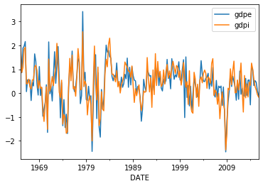
An Example: GDP+
Here I’m going to through a simple state space model described in Aruoba_2016. Since GDP data is inherently noisy, the authors use both income-side \((GDP_{It})\) and expenditure-side \((GDP_{Et})\) data on GDP growth to infer the true (unobserved) growth rate, \(GDP_t\). The authors posit that the true growth rate follows an AR(1):
\begin{align} \label{eq:gdp} GDP_t = \mu (1-\rho) + \rho GDP_{t-1} + \epsilon_t, \quad \epsilon_t \sim IID N(0, \sigma^2). \end{align}
An that both income- and expenditure-side estimates are mismeasured versions of this:
\begin{align} \label{eq:gdp-measure} \begin{array}{c} GDP_{Et} \ GDP_{It} \end{array} \bigg| GDP_t \sim IID N \left( \left[ \begin{array}{c} GDP_t \ GDP_t \end{array} \right], \left[ \begin{array}{cc} \sigma_{E}^2 & 0 \ 0 & \sigma_{I}^2 \end{array} \right]\right) \end{align}
We can cast this into state space form with \(n_y = 2\) and \(n_s = n_\epsilon = 1\). We have
\begin{align} C = \mu(1-\rho),~~ T = \rho,~~ R = 1, \mbox{ and } Q = \sigma^2, \nonumber \\\ D = \begin{bmatrix}0 \ 0 \end{bmatrix}, ~~ Z = \begin{bmatrix}1 \ 1 \end{bmatrix}, \mbox{ and } H = \left[ \begin{array}{cc} \sigma_{E}^2 & 0 \ 0 & \sigma_{I}^2 \end{array} \right]. \end{align}
Here’s a look at the data:
 We can use the Kalman filter to maximize the likelihood function,
since we haven’t quite worked out how to elicit the posterior of
this model just yet.
We can use the Kalman filter to maximize the likelihood function,
since we haven’t quite worked out how to elicit the posterior of
this model just yet.
Initial likelihood:  -4293.835439078496
      fun: 358.8810028467478
 hess_inv: <5x5 LbfgsInvHessProduct with dtype=float64>
      jac: array([-1.08002496e-04, -1.70530257e-05, -3.12638804e-04, -2.95585778e-04,
       -2.16004992e-04])
  message: b'CONVERGENCE: REL_REDUCTION_OF_F_<=_FACTR*EPSMCH'
     nfev: 108
      nit: 14
   status: 0
  success: True
        x: array([0.50974449, 0.39613152, 0.28275435, 0.40326539, 0.64044755])
Maximized Likelihood:  -358.8810028467478
{'rho': 0.5097444850915837, 'mu': 0.39613152196112617, 'sige': 0.2827543510275178, 'sigi': 0.4032653925782693, 'sig': 0.6404475458159359}
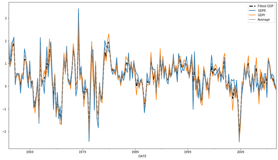
We these point estimates, we can use the kalman filter to extract \(\{ A_t\}_{t=1}^T\), the filtered means of the “true” GDP series. We’ll plot them along with the observables, and the simple average of expenditure-side and income-side GDP estimates.
To make it a bit easier to see, let’s look at the last five or so years.
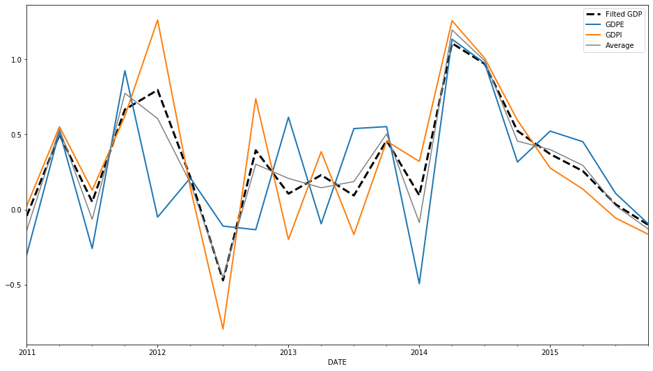 You can see the average is different form the filtered estimate.
Why is that? The Kalman Gain matrix places different weights on
the income- and expenditure-side GDP data.
You can see the average is different form the filtered estimate.
Why is that? The Kalman Gain matrix places different weights on
the income- and expenditure-side GDP data.
| 0.4217678091997104 | 0.42176780919971 |
Bibliography
References
Bibliography
[woodford_2003] Woodford, Interest and Prices, Princeton University Press (2003). ↩
[Gali2008] Jordi Gal'i, Monetary Policy, Inflation, and the Business Cycle: An Introduction to the New Keynesian Framework, Princeton University Press (2008). ↩
[ireland2004] Ireland, A Method for Taking Models to the Data, Journal of Economic Dynamics and Control, 28(6), 1205-1226 (2004). ↩
[christiano2005] Christiano, Eichenbaum, Evans & , Nominal Rigidities and the Dynamic Effects of a Shock to Monetary Policy, Journal of Political Economy, 113(1), 1-45 (2005). ↩
[Smets2007] Smets & Wouters, Shocks and Frictions in US Business Cycles: A Bayesian DSGE Approach, American Economic Review, 97, 586-608 (2007). ↩
[An2007b] An & Frank Schorfheide, Bayesian Analysis of DSGE Models, Econometric Reviews, 26(2-4), 113-172 (2007). doi. ↩
[Harvey1991] Andrew Harvey, Forecasting, Structural Time Series Models and the Kalman Filter, University of Cambridge Press (1991). ↩
[Hamilton] James Hamilton, Time Series Analysis, Princeton University Press (1994). ↩
[HerbstSchorfheide2015] Edward Herbst & Frank Schorfheide, Bayesian Estimation of DSGE Models, Princeton University Press (2015). ↩
[Fern_ndez_Villaverde_2016] Fernandez-Villaverde, Rubio-Ramirez, & Schorfheide, Solution and Estimation Methods for DSGE Models, Handbook of Macroeconomics, 527 724 (2016). link. doi. ↩
[Sims2002] Sims, Solving Linear Rational Expectations Models, Computational Economics, 20, 1-20 (2002). ↩
[DurbinKoopman2001] Durbin & Koopman, Time Series Analysis by State Space Methods, Oxford University Press (2001). ↩
[Aruoba_2016] Aruoba, Diebold, , Nalewaik, Schorfheide, Song & Dongho, Improving GDP measurement: A measurement-error perspective, Journal of Econometrics, 191(2), 384 397 (2016). link. doi. ↩